1) The document discusses the envelope theorem and its application to optimization problems with parameters. The envelope theorem describes how optimal values of decision variables change with parameters. 2) It provides an example of optimizing a quadratic function with respect to a single parameter b, showing how the optimal values of x and y vary with b. 3) The envelope theorem can be applied to constrained and unconstrained optimization problems. It allows calculating the rate of change of the optimal objective value with respect to parameters.

1. Lecturer: Farzad Javidanrad
Specific Topics in Optimisation
(for MSc & PhD Business, Management & Finance Students)
(Autumn 2014-2015)
Envelope Theorem &
Optimisation Under Intertemporal Choice

2. • Parameter: The variable that helps in defining a mathematical/statistical model but its
values are given or determined outside of the model.
In the linear model 𝑦 = 𝑚𝑥 + 𝑐,
𝑦 and 𝑥 variables (their values determined inside the model)
𝑐 and 𝑚 parameters (y-intercept and slope parameter respectively)
Basic Terminologies
Adopted and altered from http://www.met.reading.ac.uk/pplato2/h-flap/math2_2.html

3. • Objective Function: A function which is going to be optimized.
• Decision Variables: The independent (or explanatory) variables in a model.
• Optimal Values: Maximum or minimum values of variables in a model..
• The envelope theorem focus on the relation between the optimal value of the dependent
variable in a particular function and the parameter(s) of that function. How the optimal
value does change when a parameter (or one of parameters of the model) changes?
Consider the following quadratic function which contains on parameter
𝑦 = 𝑥2 − 𝑏𝑥
The optimal value of 𝑥 = 𝑥∗ can be obtained by the first order condition 𝑓′ 𝑥 = 0:
2𝑥 − 𝑏 = 0 → 𝑥∗ =
𝑏
2
and 𝑦∗ = 𝑥∗2
− 𝑏𝑥∗ ⟹ 𝑦∗ = −
𝑏2
4
Obviously, 𝑥∗ and consequently, 𝑦∗ are functions of 𝑏, i.e. 𝑥∗ = 𝑥 𝑏 , 𝑦∗ = 𝑦(𝑏).
Basic Terminologies

4. • The following table shows how the optimal values of 𝑥 and 𝑦 change when 𝑏 changes.
Investigate how the optimal value of the dependent variable in the quadratic function
𝑦 = 𝑎𝑥2 + 𝑏𝑥 + 𝑐 changes when each parameter 𝑎, 𝑏 and 𝑐 change.
Basic Example
𝒃
𝒙∗
=
𝒃
𝟐
𝒚∗
= −
𝒃 𝟐
𝟒
-2 -1 -1
-1 -0.5 -0.25
0 0 0
1 0.5 -0.25
2 1 -1 -1.2
-1
-0.8
-0.6
-0.4
-0.2
0
-3 -2 -1 0 1 2 3
b
𝒚

5. • Case 1 (unconstraint model): Consider a general optimization model with two independent
(decision) variables 𝑥 and 𝑦 and one parameter 𝛼:
𝑧 = 𝑓(𝑥, 𝑦, 𝛼)
The first-order necessary conditions are:
𝜕𝑧
𝜕𝑥
= 𝑓𝑥 = 0 𝑎𝑛𝑑
𝜕𝑧
𝜕𝑦
= 𝑓𝑦 = 0
Assume the second-order conditions hold, the optimal values of 𝑥 and 𝑦 for any given value
of 𝛼 are the function of 𝛼, i.e. 𝑥∗ = 𝑥∗ (𝛼) and 𝑦∗ = 𝑦∗ 𝛼 . By substituting these optimal
values into the objective function we obtain the indirect objective function, which is an
indirect function of the parameter 𝛼 :
𝜑 𝛼 = 𝑓(𝑥∗ 𝛼 , 𝑦∗ 𝛼 , 𝛼)
The Envelope Theorem (Unconstraint Model)
Objective function with two decision variables and
one parameter
𝜑 𝛼 gives the optimal value of 𝑧, for any given
value of 𝛼

6. • Some of the properties of the indirect objective functions are:
A. For any given set of parameters, the objective function is optimized (maximized or
minimized)
B. When the parameters vary, the indirect objective function outlines the optimum values
of the direct objective function.
C. The graph of the indirect objective function is an envelope of the graphs of optimized
objective functions when parameters vary.
• In order to find the variation of indirect objective function 𝜑 𝛼 in terms of 𝛼, we need to
differentiate it:
The Envelope Theorem (Unconstraint Model)

7. 𝜕𝜑
𝜕𝛼
= 𝑓𝑥
𝜕𝑥∗
𝜕𝛼
+ 𝑓𝑦
𝜕𝑦∗
𝜕𝛼
+ 𝑓𝛼
However, we know that at the optimal values 𝑓𝑥 = 𝑓𝑦 = 0, so:
𝜕𝜑
𝜕𝛼
= 𝑓𝛼
This equation says that the rate of change of the optimal value of the dependent variable 𝑧 in
terms of 𝛼, where the independent variables 𝑥 and 𝑦 are optimally obtained (for any given
𝛼), can be calculated directly by differentiating the indirect objective function 𝜑 in terms of 𝛼.
• Geometric Interpretation: If we plot 𝜑 𝛼 for various 𝛼′ 𝑠,
the plot will be the envelope of the different curves obtained
from the family function 𝑧 = 𝑓(𝑥, 𝑦, 𝛼), when 𝛼 changes.
• Here we have a function with one variable and one parameter.
The Envelope Theorem (Unconstraint Model)
𝑧 = 𝑓(𝑥, 𝛼)
𝛼 𝑥∗
(𝛼)
𝜑 𝛼
Adoptedand altered from http://exactitude.tistory.com/229.

8. Economic Example
• Here we have the relation between short-run (SR) and long-run (LR) average cost curves when the
size of production (parameter)
changes.
• The long-run average cost (LRAC) is the envelope
curve for different short-run average cost (SRAC)
curves when the size of the company changes in
the long-run.
• The theorem can be generalised to include more than one parameter. For example, in
microeconomics, a price-taker producer face with the following profit function:
𝜋 = 𝑝. 𝑓 𝐿, 𝐾 − 𝑤𝐿 − 𝑟𝐾
Where 𝑝 is the output price, 𝑤 and 𝑟 are factor production prices or simply the cost of employing
labour and capital in the production process. They are parameters of the model.
Size of the company (production) increasing
Adoptedandalteredfromhttp://maaw.info/EconomiesOfScaleNote.htm
= 𝜑 𝛼

9. • To know how profit 𝜋 changes when one of these parameters change, say 𝑤, we can simply
differentiate the objective function with respect to that parameter, assuming other
parameters and variables constant, i.e.:
𝜕𝜋
𝜕𝑤
= −𝐿
• Using the envelope theorem leads us to the same result but 𝐿 should be evaluated at its
optimal value, 𝐿∗ (the value that maximise 𝜋 at any given values of 𝑝, 𝑤 and 𝑟 ), because:
Through profit maximising we reach to the optimal level of demand for labour and capital as:
𝐿∗
= 𝐿∗
𝑝, 𝑤, 𝑟 𝑎𝑛𝑑 𝐾∗
= 𝐾∗
(𝑝, 𝑤, 𝑟)
So, the indirect profit function will be:
𝜋∗
𝑝, 𝑤, 𝑟 = 𝑝. 𝑓 𝐿∗
, 𝐾∗
− 𝑤𝐿∗
− 𝑟𝐾∗
Now,
𝜕𝜋∗
𝜕𝑤
= 𝑝 𝑓𝐿
𝜕𝐿∗
𝜕𝑤
+ 𝑓𝐾
𝜕𝐾∗
𝜕𝑤
− 𝑤
𝜕𝐿∗
𝜕𝑤
− 𝐿∗
− 𝑟
𝜕𝐾∗
𝜕𝑤
𝜕𝜋∗
𝜕𝑤
= 𝑝𝑓𝐿 − 𝑤
𝜕𝐿∗
𝜕𝑤
+ 𝑝𝑓𝐾 − 𝑟
𝜕𝐾∗
𝜕𝑤
− 𝐿∗
Knowing that at the optimal values of 𝐿 and 𝐾 the terms in parentheses are zero, therefore, we will reach to:
𝜕𝜋∗
𝜕𝑤
= −𝐿∗
The Envelope Theorem (Unconstraint Model)
 This means if this particular employer faces
with the increase in wage rate by £1, in case
he/she has employed 1000 workers and this is
the optimal level of labour which makes the
maximum profit, he/she will lose -£1000 by £1
increase in the wage.
 A profit-maximising firm, in this situation
would reduce the number of workers up to a
point that the increase in cost is compensated
by reduce in payment in total.

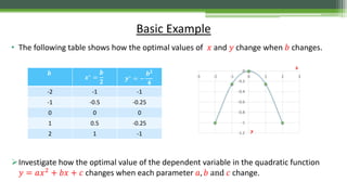
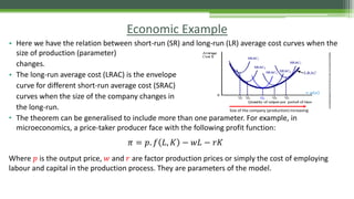
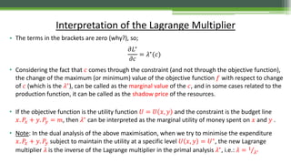
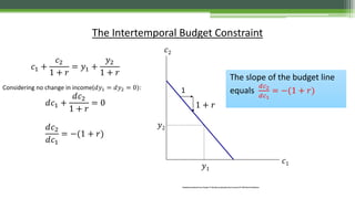
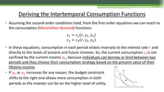
10. • Case 2 (constraint model): It rarely happens to optimise a function without any constraint. In the real
world any optimisation is subject to one or more constraints. Again, imagine a simple example of
optimisation with two independent variables and one parameter 𝛼:
𝑍 = 𝑓(𝑥, 𝑦, 𝛼)
Subject to the constraint
𝑔 𝑥, 𝑦, 𝛼 = 𝑐
The Lagrangian Function can be written as:
𝐿(𝑥, 𝑦, 𝜆, 𝛼) = 𝑓 𝑥, 𝑦, 𝛼 + 𝜆[𝑐 − 𝑔 𝑥, 𝑦, 𝛼 ]
Setting the first partial derivatives of 𝐿 equal to zero,
𝐿 𝑥 = 𝑓𝑥 − 𝜆𝑔 𝑥 = 0
𝐿 𝑦 = 𝑓𝑦 − 𝜆𝑔 𝑦 = 0
𝐿 𝜆 = 𝑔(𝑥, 𝑦, 𝛼) = 𝑐
Assuming the second-order conditions are satisfied, solving these equations gives the optimal values of
𝑥, 𝑦 and 𝜆, in terms of the parameter 𝛼.
The Envelope Theorem (Constraint Model)
A
𝑐 is a constant
𝜆 is the Lagrange
Multiplier

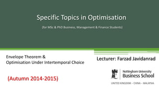
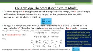
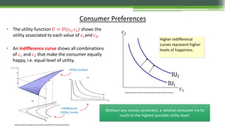
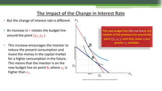
11. 𝑥∗
= 𝑥∗
(𝛼)
𝑦∗
= 𝑦∗
(𝛼)
𝜆∗
= 𝜆∗
(𝛼)
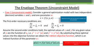
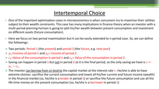
And the indirect objective function will be:
𝑍∗ = 𝑓 𝑥∗ 𝛼 , 𝑦∗ 𝛼 , 𝛼 = 𝜑(𝛼)
𝜑(𝛼) is the maximum value of 𝑍 for all values of 𝑥 and 𝑦 that satisfy the constraint and also it shows
the maximum value of 𝑍 for any value of 𝛼.
How does 𝜑(𝛼) change when 𝛼 changes? To answer this, we need somehow to consider the
constraint function 𝑔 𝑥, 𝑦, 𝛼 = 𝑐 in our analysis. To do that, we make indirect Lagrangian function 𝐿∗
, using
optimal values 𝑥∗
and 𝑦∗
and then differentiate the new indirect function with respect to 𝛼.
𝐿∗ 𝑥∗ 𝛼 , 𝑦∗ 𝛼 , 𝜆, 𝛼 = 𝜑 𝛼 + 𝜆[𝑐 − 𝑔 𝑥∗ 𝛼 , 𝑦∗ 𝛼 , 𝛼 ]
By maximising 𝐿∗
we have, in fact, maximised 𝜑 𝛼 , why?
The Envelope Theorem (Constraint Model)
Indirect objective
function
= 0

12. • By differentiating 𝐿∗
with respect to 𝛼 we have:
𝜕𝐿∗
𝜕𝛼
= 𝑓𝑥 − 𝜆𝑔 𝑥
𝜕𝑥∗
𝜕𝛼
+ 𝑓𝑦 − 𝜆𝑔 𝑦
𝜕𝑦∗
𝜕𝛼
+ 𝑓𝛼 − 𝜆𝑔 𝛼
Or
𝜕𝐿∗
𝜕𝛼
= 𝐿 𝑥
𝜕𝑥∗
𝜕𝛼
+ 𝐿 𝑦
𝜕𝑦∗
𝜕𝛼
+ 𝐿 𝛼
Where 𝐿𝑖 is the partial derivative of the Lagrangian function with respect to element 𝑖.
Base on the first order conditions , 𝐿 𝑥 and 𝐿 𝑦 are zero, then:
𝜕𝐿∗
𝜕𝛼
= 𝐿 𝛼 = 𝑓𝛼 − 𝜆𝑔 𝛼
• Using the Lagrange method allow us to change the optimisation of a constraint model to the
optimisation of an unconstraint model.
• Note: If the parameter enters just in the objective function the result for constraint and unconstraint
models are similar.
The Envelope Theorem (Constraint Model)
A

13. • Solving the first two equations of , simultaneously (by ignoring 𝛼, which means considering it as
a fixed value without any variation), gives the value of 𝜆 as:
𝜆 =
𝑓𝑥
𝑔 𝑥
=
𝑓𝑦
𝑔 𝑦
By re-arranging the terms, we will have:
𝜆 =
𝑓𝑥
𝑓𝑦
=
𝑔 𝑥
𝑔 𝑦
This means 𝜆 is the slope of the level curve of the objective function 𝑓(𝑥, 𝑦) at the optimal points
𝑥∗and 𝑦∗, which should be equal to the slope of the level curve of the constraint function 𝑔(𝑥, 𝑦) at
those points.
Interpretation of the Lagrange Multiplier
A
Both picturesadopted from http://en.wikipedia.org/wiki/Lagrange_multiplier

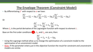
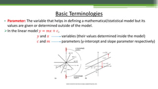
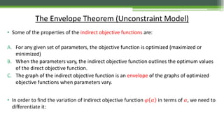
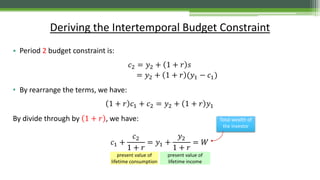
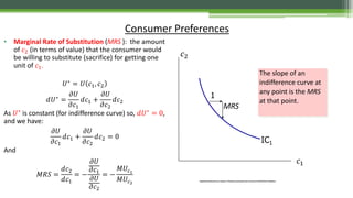
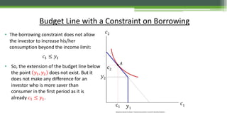
14. • But more information about 𝜆 can be obtained through the envelope theorem:
By solving all equations in simultaneously (again consider 𝛼 as a constant), the optimal values for
variables and 𝜆 will be:
𝑥∗
= 𝑥∗
𝑐 , 𝑦∗
= 𝑦∗
𝑐 , 𝜆∗
= 𝜆∗
𝑐
Substituting these results into the Lagrangian function 𝐿(𝑥, 𝑦, 𝜆), we have:
𝐿∗ 𝑥∗ 𝑐 , 𝑦∗ 𝑐 , 𝜆∗ 𝑐 = 𝑓 𝑥∗ 𝑐 , 𝑦∗ 𝑐 , 𝜆∗ 𝑐 + 𝜆∗ 𝑐 [𝑐 − 𝑔 𝑥∗ 𝑐 , 𝑦∗ 𝑐 ]
Differentiating with respect to 𝑐, we have:
𝜕𝐿∗
𝜕𝑐
= 𝑓𝑥
𝜕𝑥∗
𝜕𝑐
+ 𝑓𝑦
𝜕𝑦∗
𝜕𝑐
+ 𝑐 − 𝑔 𝑥∗, 𝑦∗
𝜕𝜆∗
𝜕𝑐
+ 𝜆∗ [1 − 𝑔 𝑥
𝜕𝑥∗
𝜕𝑐
− 𝑔 𝑦
𝜕𝑦∗
𝜕𝑐
]
By rearranging, we get:
𝜕𝐿∗
𝜕𝑐
= 𝑓𝑥 − 𝜆∗
𝑔 𝑥
𝜕𝑥∗
𝜕𝑐
+ 𝑓𝑦 − 𝜆∗
𝑔 𝑦
𝜕𝑦∗
𝜕𝑐
+ 𝑐 − 𝑔 𝑥∗
, 𝑦∗
𝜕𝜆∗
𝜕𝑐
+ 𝜆∗
Interpretation of the Lagrange Multiplier
A

15. • The terms in the brackets are zero (why?), so;
𝜕𝐿∗
𝜕𝑐
= 𝜆∗(𝑐)
• Considering the fact that 𝑐 comes through the constraint (and not through the objective function),
the change of the maximum (or minimum) value of the objective function 𝑓 with respect to change
of 𝑐 (which is the 𝜆∗), can be called as the marginal value of the 𝑐, and in some cases related to the
production function, it can be called as the shadow price of the resources.
• If the objective function is the utility function 𝑈 = 𝑈 𝑥, 𝑦 and the constraint is the budget line
𝑥. 𝑃𝑥 + 𝑦. 𝑃𝑦 = 𝑚, then 𝜆∗
can be interpreted as the marginal utility of money spent on 𝑥 and 𝑦 .
• Note: In the dual analysis of the above maximisation, when we try to minimise the expenditure
𝑥. 𝑃𝑥 + 𝑦. 𝑃𝑦 subject to maintain the utility at a specific level 𝑈 𝑥, 𝑦 = 𝑈∗
, the new Lagrange
multiplier 𝜆 is the inverse of the Lagrange multiplier in the primal analysis 𝜆∗, i.e.: 𝜆 = 1
𝜆∗
Interpretation of the Lagrange Multiplier

16. • One of the important optimisation cases in microeconomics is when consumers try to maximise their utilities
subject to their wealth constraints. This case has many implications in finance theory when an investor with a
multi-period planning horizon is going to split his/her wealth between present consumption and investment
on different assets (future consumption).
• Here we focus on two period maximization but it can be easily extended to n-period case. So, we can define
the followings:
 Two periods: Period 1 (the present) and period 2 (the future, e.g. next year)
 𝑦1=Income of period 1 and 𝑦2= Income of period 2
 𝑐1=Value of the consumption in period 1 and 𝑐2= Value of the consumption in period 2
 Saving can happen in period 1 but not in period 2 as it is the final period, so the only saving we have is 𝑠 =
𝑦1 − 𝑐1.
 The investor can borrow from or lend to the capital market at the interest rate 𝑟. He/she is able to have
extreme choices: sacrifice the current consumption and invest all his/her current and future income (wealth)
in the financial market (so, he/she is a lender in period 1) or sacrifice the future consumption and use all the
life-time money on the present consumption (so, he/she is a borrower in period 1)
Intertemporal Choice

17. Deriving the Intertemporal Budget Constraint
• Period 2 budget constraint is:
𝑐2 = 𝑦2 + 1 + 𝑟 𝑠
= 𝑦2 + 1 + 𝑟 (𝑦1 − 𝑐1)
• By rearrange the terms, we have:
1 + 𝑟 𝑐1 + 𝑐2 = 𝑦2 + 1 + 𝑟 𝑦1
By divide through by 1 + 𝑟 , we have:
𝑐1 +
𝑐2
1 + 𝑟
= 𝑦1 +
𝑦2
1 + 𝑟
= 𝑊
present value of
lifetime consumption
present value of
lifetime income
Total wealth of
the investor

18. The Intertemporal Budget Constraint
• The budget constraint
shows all combinations
of 𝑐1and 𝑐2that just
exhaust the consumer’s
resources.
𝑐1
𝑐2
𝑦1
𝑦2
Borrowing
Saving
Consumption = income (in
both periods)
The point ( 𝑦1, 𝑦2) is always on the
budget line because 𝑐1= 𝑦1, 𝑐2= 𝑦2
• The Budget Constraint:
𝑐1 +
𝑐2
1 + 𝑟
= 𝑦1 +
𝑦2
1 + 𝑟
Or
(𝑦1−𝑐1) +
𝑦2 − 𝑐2
1 + 𝑟
= 0
𝑦2 + 1 + 𝑟 𝑦1
𝑦1 +
𝑦2
1 + 𝑟
Adoptedand altered from Chapter17 Mankiw producedby Ron Cronovich © 2010 Worth Publishers

19. The Intertemporal Budget Constraint
The slope of the budget line
equals
𝑑𝑐2
𝑑𝑐1
= −(1 + 𝑟)
𝑐1
𝑐2
𝑦1
𝑦2
1
𝑐1 +
𝑐2
1 + 𝑟
= 𝑦1 +
𝑦2
1 + 𝑟
Considering no change in income(𝑑𝑦1 = 𝑑𝑦2 = 0):
𝑑𝑐1 +
𝑑𝑐2
1 + 𝑟
= 0
𝑑𝑐2
𝑑𝑐1
= −(1 + 𝑟)
1 + 𝑟
Adoptedand altered from Chapter17 Mankiw producedby Ron Cronovich © 2010 Worth Publishers

20. Consumer Preferences
• The utility function 𝑈 = 𝑈(𝑐1, 𝑐2) shows the
utility associated to each value of 𝑐1and 𝑐2.
• An indifference curve shows all combinations
of 𝑐1 and 𝑐2 that make the consumer equally
happy, i.e. equal level of utility.
𝑐1
𝑐2
IU1
IU2
Higher indifference
curves represent higher
levels of happiness.
Adoptedfrom http://www.cengage.com/economics/book_content/032427470X_nechyba/chapters/partA.html
Adoptedand altered from Chapter17 Mankiw producedby Ron Cronovich © 2010 Worth Publishers
Without any money constraint, a rational consumer try to
reach to the highest possible utility level.
Utility Surface
Indifference
Utility Curves

21. • Marginal Rate of Substitution (MRS ): the amount
of 𝑐2 (in terms of value) that the consumer would
be willing to substitute (sacrifice) for getting one
unit of 𝑐1.
𝑈∗
= 𝑈 𝑐1, 𝑐2
𝑑𝑈∗ =
𝜕𝑈
𝜕𝑐1
𝑑𝑐1 +
𝜕𝑈
𝜕𝑐2
𝑑𝑐2
As 𝑈∗
is constant (for indifference curve) so, 𝑑𝑈∗
= 0,
and we have:
𝜕𝑈
𝜕𝑐1
𝑑𝑐1 +
𝜕𝑈
𝜕𝑐2
𝑑𝑐2 = 0
And
𝑀𝑅𝑆 =
𝑑𝑐2
𝑑𝑐1
= −
𝜕𝑈
𝜕𝑐1
𝜕𝑈
𝜕𝑐2
= −
𝑀𝑈𝑐1
𝑀𝑈𝑐2
IC1
The slope of an
indifference curve at
any point is the MRS
at that point.
1
MRS
Consumer Preferences
Adoptedand altered from Chapter17 Mankiw producedby Ron Cronovich © 2010 Worth Publishers
𝑐1
𝑐2

22. Optimization
• The optimal O( 𝑐1, 𝑐2) is where the
budget line just touches the highest
indifference curve.
• At the optimal point the slope of the
indifference curve is equal to the
slope of the budget line.
𝑐1
𝑐2
O
At the optimal point,
MRS = −(1 + 𝑟)
Adoptedfrom http://www2.hawaii.edu/~fuleky/anatomy/anatomy.html
Adoptedand altered from Chapter17 Mankiw producedby Ron Cronovich © 2010 Worth Publishers

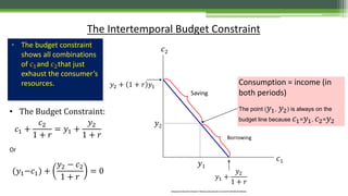
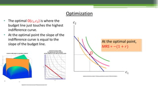
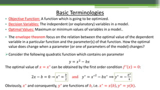
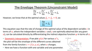
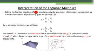
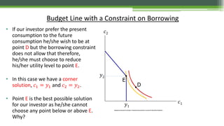
23. Maximisation of the Intertemporal Utility
• Maximise: 𝑈 = 𝑈(𝑐1, 𝑐2) , subject to:(𝑦1−𝑐1) +
𝑦2−𝑐2
1+𝑟
= 0
• The Lagrange function for this problem is:
𝐿 𝑐1, 𝑐2, λ = 𝑈 𝑐1, 𝑐2 + λ[(𝑦1−𝑐1) +
𝑦2 − 𝑐2
1 + 𝑟
]
Producing the first-order conditions:
𝐿1 =
𝜕𝑈
𝜕𝑐1
− 𝜆 = 0
𝐿2 =
𝜕𝑈
𝜕𝑐2
−
𝜆
1 + 𝑟
= 0
𝐿 𝜆 = (𝑦1−𝑐1) +
𝑦2 − 𝑐2
1 + 𝑟
= 0
Solving for the first two equations:
𝜕𝑈
𝜕𝑐1
𝜕𝑈
𝜕𝑐2
= 1 + 𝑟 ⟹
𝑀𝑈𝑐1
𝑀𝑈𝑐2
= 1 + 𝑟
In the optimal point the slope of the
indifference curve should be equal to the
slope of the constraint.

24. • Assuming the second-order conditions hold, from the first-order equations we can reach to
the consumption (Marshallian demand) functions:
𝑐1 = 𝑐1 𝑟, 𝑦1, 𝑦2
𝑐2 = 𝑐2 𝑟, 𝑦1, 𝑦2
• In these equations, consumption in each period relates inversely to the interest rate 𝑟 and
directly to the levels of present and future incomes. So, the current consumption 𝑐1is not
confined by the current income 𝑦1, because individuals can borrow or lend between two
periods and they choose their consumption strategy based on the present value of their
lifetime income.
• If 𝑦1 or 𝑦2 increases for any reason, the budget constraint
shifts to the right and allows more consumption in both
periods as the investor can be on the higher level of utility.
Deriving the Intertemporal Consumption Functions
𝑐1
𝑐2

25. A
The Impact of the Change in Interest Rate
𝑐1
𝑐2
𝑦1
𝑦2
A
B
• But the change of interest rate is different.
• An increase in 𝑟 rotates the budget line
around the point (𝑦1, 𝑦2 ).
• This increase encourages the investor to
reduce the present consumption and
invest the money in the capital market
for a higher consumption in the future.
This means that the investor is on the
new budget line on point B, where 𝑐2 is
higher than 𝑐1.
Adoptedand altered from Chapter17 Mankiw producedby Ron Cronovich © 2010 Worth Publishers
The new budget line (the red line)is the
rotation of the previous line around the
point (𝑦1, 𝑦2 ), such that, lesser 𝑐1but
greater 𝑐2 available.

26. Budget Line with a Constraint on Borrowing
𝑐1
𝑐2
𝑦1
𝑦2
• The borrowing constraint does not allow
the investor to increase his/her
consumption beyond the income limit:
𝑐1 ≤ 𝑦1
• So, the extension of the budget line below
the point 𝑦1, 𝑦2 does not exist. But it
does not make any difference for an
investor who is more saver than
consumer in the first period as it is
already 𝑐1 ≤ 𝑦1.
c1
c2
𝐴
Adoptedand altered from Chapter17 Mankiw producedby Ron Cronovich © 2010 Worth Publishers

27. Budget Line with a Constraint on Borrowing
• If our investor prefer the present
consumption to the future
consumption he/she wish to be at
point D but the borrowing constraint
does not allow that therefore,
he/she must choose to reduce
his/her utility level to point E.
• In this case we have a corner
solution, 𝑐1 = 𝑦1 and 𝑐2 = 𝑦2.
• Point E is the best possible solution
for our investor as he/she cannot
choose any point below or above E.
Why?
𝑐1
𝑐2
𝑦1
D
E
𝑦2
Adoptedand altered from Chapter17 Mankiw producedby Ron Cronovich © 2010 Worth Publishers