This document provides an in-depth explanation of simple linear regression (SLR), including its mathematical formulation, estimation of model parameters, significance testing, and goodness of fit. It explains how to derive the model parameters β0 and β1 using sample data, the principle of least squares, and describes the processes for testing the significance of these parameters. Additionally, it covers the coefficient of determination (r²) as a measure of the model's explanatory power.
![Simple Linear Regression
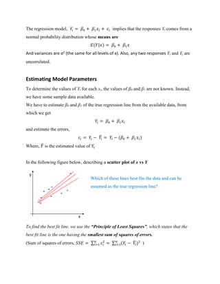
The simplest of all machine learning techniques is “Simple Linear Regression”. In this
blog, I will explain in detail the mathematical formulation of Simple Linear Regression
(SLR) and how to:
• Estimate model parameters
• Test significance of parameters
• Test goodness of the model fit
Let me begin with the definition of SLR. A simple linear regression is a statistical
technique used to investigate the relationship between two variables in a non-
deterministic fashion. In general, it is used to estimate an unknown variable (aka
dependent variable) by determining its relationship with a known variable (aka
independent variable).
Model Formulation
An SLR model can be generalized as:
𝑌 = 𝛽0 + 𝛽1 𝑥 + 𝜀
where, Y – dependent variable
x – independent variable
ε – random error [we assume ε ~ N(0, σ2
), homogenous and uncorrelated]
β0 – intercept (value of Y, when x = 0)
β1 – slope (change in Y per unit change in x)
An SLR model has 2 components,
• Deterministic (β0 + β1x)
• Random / Non-deterministic (ε)
This random error (ε) characterizes the linear regression model.](https://image.slidesharecdn.com/slr-180708185345/85/Simple-Linear-Regression-1-320.jpg)
![Simple Linear Regression
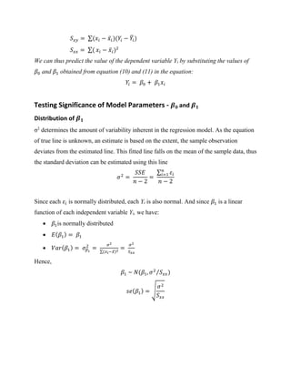
The simplest of all machine learning techniques is “Simple Linear Regression”. In this
blog, I will explain in detail the mathematical formulation of Simple Linear Regression
(SLR) and how to:
• Estimate model parameters
• Test significance of parameters
• Test goodness of the model fit
Let me begin with the definition of SLR. A simple linear regression is a statistical
technique used to investigate the relationship between two variables in a non-
deterministic fashion. In general, it is used to estimate an unknown variable (aka
dependent variable) by determining its relationship with a known variable (aka
independent variable).
Model Formulation
An SLR model can be generalized as:
𝑌 = 𝛽0 + 𝛽1 𝑥 + 𝜀
where, Y – dependent variable
x – independent variable
ε – random error [we assume ε ~ N(0, σ2
), homogenous and uncorrelated]
β0 – intercept (value of Y, when x = 0)
β1 – slope (change in Y per unit change in x)
An SLR model has 2 components,
• Deterministic (β0 + β1x)
• Random / Non-deterministic (ε)
This random error (ε) characterizes the linear regression model.](https://image.slidesharecdn.com/slr-180708185345/75/Simple-Linear-Regression-1-2048.jpg)
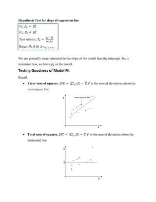
![Thus, to obtain β0 and β1 of the best fit line
𝑌𝑖 = 𝛽0 + 𝛽1 𝑥𝑖
we minimize,
𝑓( 𝛽0, 𝛽1) = ∑ 𝜀𝑖
2𝑛
𝑖=1 = ∑ (𝑌𝑖 − 𝑌̂𝑖)2𝑛
𝑖=1 = ∑ (𝑌𝑖 − 𝛽0 − 𝛽1 𝑥𝑖)2𝑛
𝑖=1 …(1)
To find the minimum of equation (1), partially differentiate 𝑓( 𝛽0, 𝛽1) with respect to β0
and β1 and equate to zero.
𝜕𝑓
𝜕𝑥
= −2 ∑( 𝑌𝑖 − 𝛽0 − 𝛽1 𝑥𝑖) = 0 … (2)
⇒ 𝛽0 𝑛 + 𝛽1 ∑ 𝑥𝑖 = ∑ 𝑦𝑖 … (3)
𝜕𝑓
𝜕𝑥
= −2 ∑( 𝑌𝑖 − 𝛽0 − 𝛽1 𝑥𝑖) = 0 … (4)
⇒ 𝛽0 ∑ 𝑥𝑖 + 𝛽1 ∑ 𝑥𝑖
2
= ∑ 𝑥𝑖 𝑦𝑖 … (5)
Solve equations (3) and (5) to obtain β0 and β1.
Equations (3) and (5) in matrix form:
[
𝑛 ∑ 𝑥𝑖
∑ 𝑥𝑖 ∑ 𝑥𝑖
2] . [
𝛽0
𝛽1
] = [
∑ 𝑥𝑖
∑ 𝑥𝑖 𝑌𝑖
] … (6)
[
𝛽0
𝛽1
] = [
𝑛 ∑ 𝑥𝑖
∑ 𝑥𝑖 ∑ 𝑥𝑖
2]
−1
. [
∑ 𝑥𝑖
∑ 𝑥𝑖 𝑌𝑖
] … (7)
[
𝛽0
𝛽1
] =
1
𝑛 ∑ 𝑥 𝑖
2− (∑ 𝑥 𝑖)2
[
∑ 𝑥𝑖
2
∑ 𝑌𝑖 − ∑ 𝑥𝑖 ∑ 𝑥𝑖 𝑌𝑖
𝑛 ∑ 𝑥𝑖 𝑌𝑖 − ∑ 𝑥𝑖 ∑ 𝑥𝑖 𝑌𝑖
] … (8)
From equation (8),
𝛽1 =
∑ 𝑥 𝑖 𝑌 𝑖−
∑ 𝑥 𝑖 ∑ 𝑌 𝑖
𝑛
∑ 𝑥 𝑖
2−
(∑ 𝑥 𝑖)2
𝑛
… (9)
𝛽1 =
∑(𝑥 𝑖−𝑥̅ 𝑖)(𝑌 𝑖−𝑌̅ 𝑖)
∑(𝑥 𝑖−𝑥̅ 𝑖)2
=
𝑆 𝑥𝑦
𝑆 𝑥𝑥
… (10)
𝛽0 = 𝑌̅ − 𝛽1 𝑥̅ … (11)
where, 𝑥̅ =
∑ 𝑥 𝑖
𝑛
𝑌̅ =
∑ 𝑌 𝑖
𝑛](https://image.slidesharecdn.com/slr-180708185345/85/Simple-Linear-Regression-3-320.jpg)
![The assumptions of SLR model states that:
𝜷 𝟏− 𝜷 𝟏
𝟎
√𝝈 𝜷 𝟏
𝟐
~ 𝑵( 𝟎, 𝟏)
Thus, the standardized variable:
𝑇 =
𝛽1 − 𝛽1
0
𝜎 √ 𝑆 𝑥𝑥⁄
=
𝛽1 − 𝛽1
0
𝑠𝑒( 𝛽1)
has a t – distribution with (n-2) degrees of freedom.
Hypothesis Test for slope of regression line:
𝐻0: 𝛽1 = 𝛽1
0
𝐻 𝛼: 𝛽1 ≠ 𝛽1
0
Test statistic, 𝑇0 =
𝛽1− 𝛽1
0
𝑠𝑒(𝛽1)
Reject H0 if | 𝑡| ≥ 𝑡 𝛼 2 ,𝑛−2⁄
The most general assumption is 𝐻0: 𝛽1 = 0 versus 𝐻 𝛼: 𝛽1 ≠ 0
In this case, rejecting H0 implies that there is no significant relation between x and Y.
Distribution of 𝜷 𝟎
Using a similar approach as that of 𝛽1, we get,
𝛽0 ~ 𝑁(𝛽0, 𝜎𝛽0
2
)
where, 𝜎𝛽0
2
= 𝜎2
[
1
𝑛
+
𝑥̅2
∑(𝑥 𝑖− 𝑥̅)2
] = 𝜎2
[
1
𝑛
+
𝑥̅2
𝑆 𝑥𝑥
]
Also,
𝜷 𝟎− 𝜷 𝟎
𝟎
√𝝈 𝜷 𝟎
𝟐
~ 𝑵( 𝟎, 𝟏)
Thus, the standardized variable,
𝑇 =
𝛽0 − 𝛽0
0
𝑠𝑒( 𝛽0)
has a t – distribution with (n-2) degrees of freedom](https://image.slidesharecdn.com/slr-180708185345/85/Simple-Linear-Regression-5-320.jpg)


![제 23회 보아즈(BOAZ) 빅데이터 컨퍼런스 - [MBOAX] : ABSA를 활용한 소비자 반응 분석 기반 운영 효율화 대시보드 설계](https://cdn.slidesharecdn.com/ss_thumbnails/3-1boaz23rdconferencemboax-260203102709-9d519923-thumbnail.jpg?width=640&height=640&fit=bounds)


