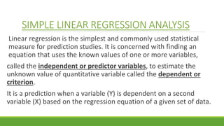
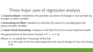
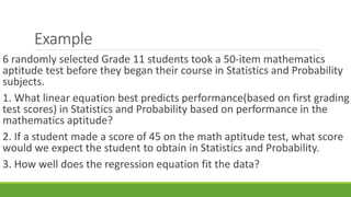
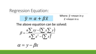
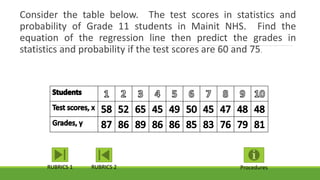
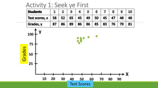
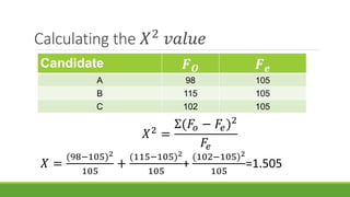
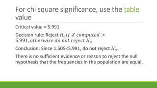
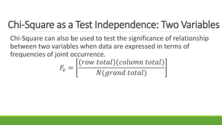
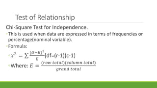
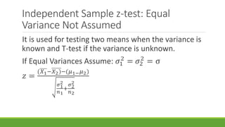
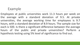
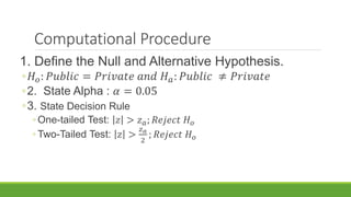
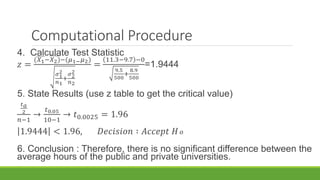
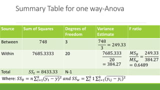
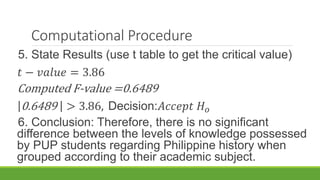
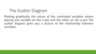
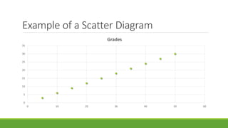
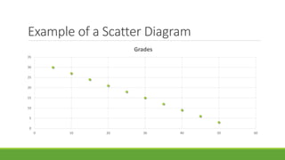
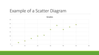
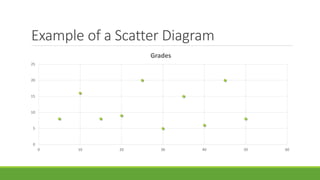
The document discusses statistical techniques for analyzing data, including scatter diagrams, correlation coefficients, regression analysis, and chi-square tests. It provides examples of using scatter diagrams to visualize the relationship between two variables, calculating the Pearson correlation coefficient to determine the strength of linear relationships, and using simple linear regression to find the regression equation that best predicts a dependent variable from an independent variable. It also explains how to perform a chi-square test to analyze relationships between categorical variables by comparing observed and expected frequencies.
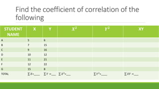
![Pearson r Formula:
𝑟 =
𝑛 𝑥𝑦− 𝑥 𝑦
[𝑛 𝑥2−( 𝑥)
2
][𝑛 𝑦2−( 𝑦)
2
]](https://image.slidesharecdn.com/lesson27usingstatisticaltechniquesinanalyzingdata-181008231053/85/Lesson-27-using-statistical-techniques-in-analyzing-data-12-320.jpg)