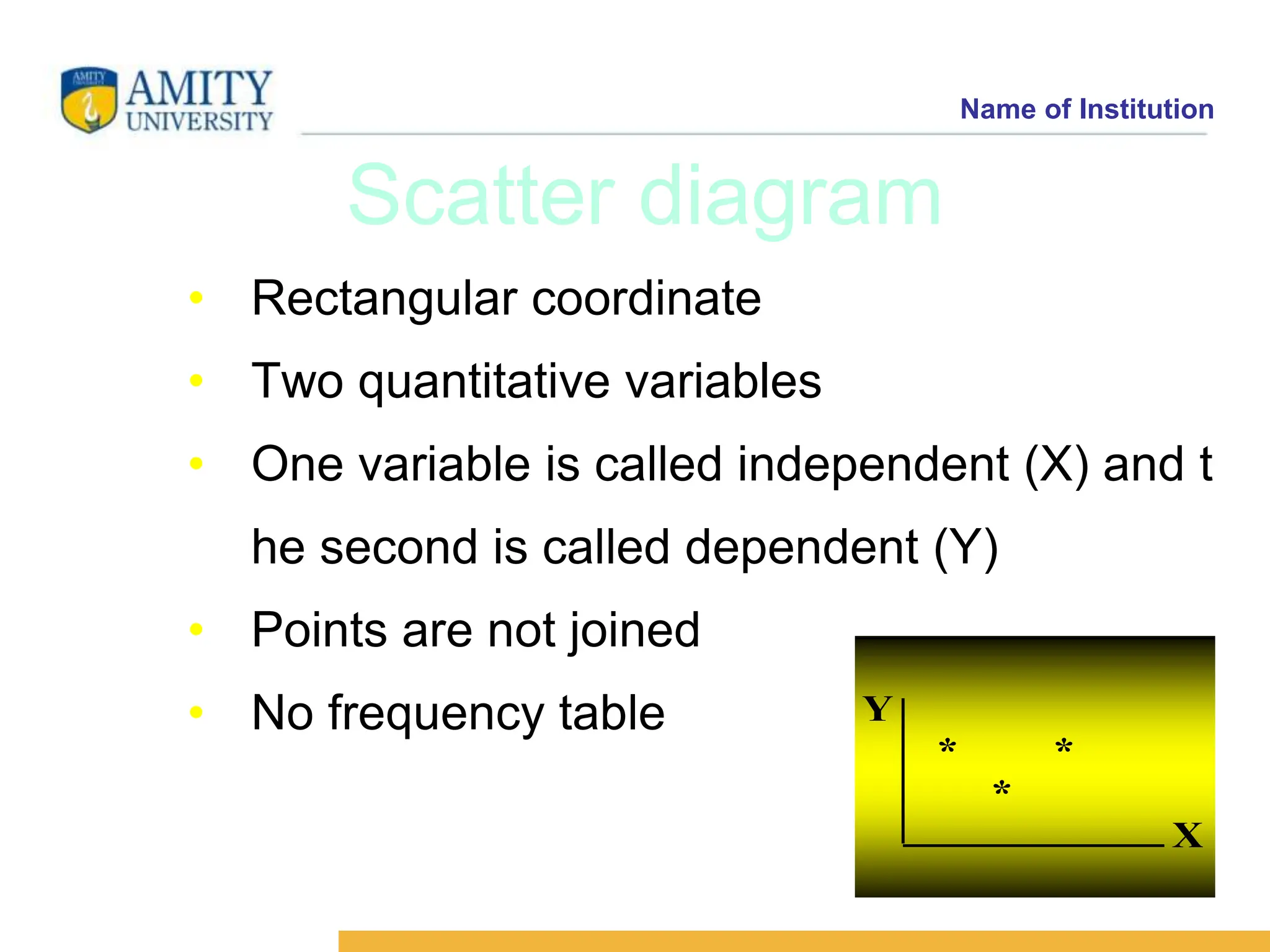
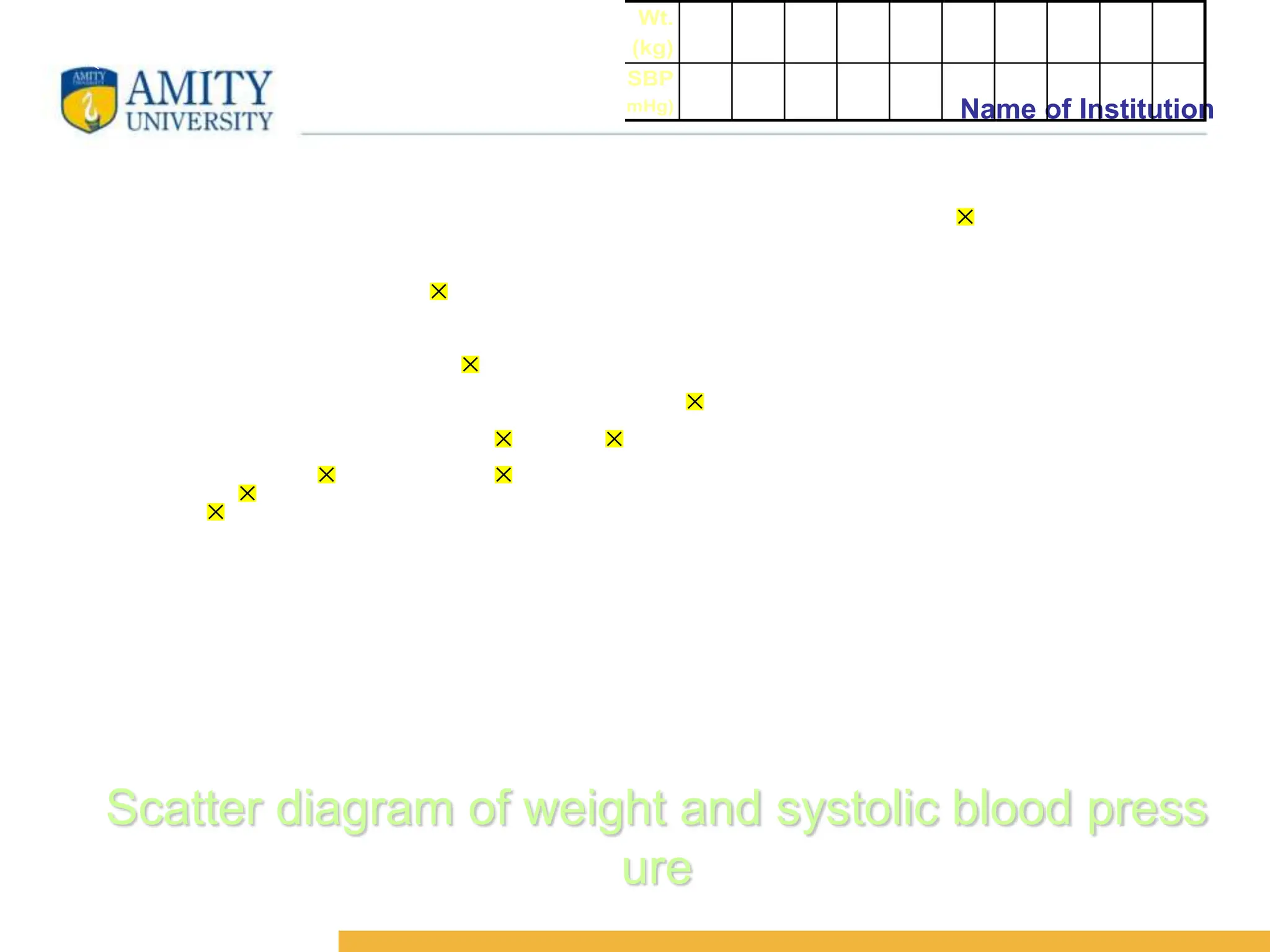
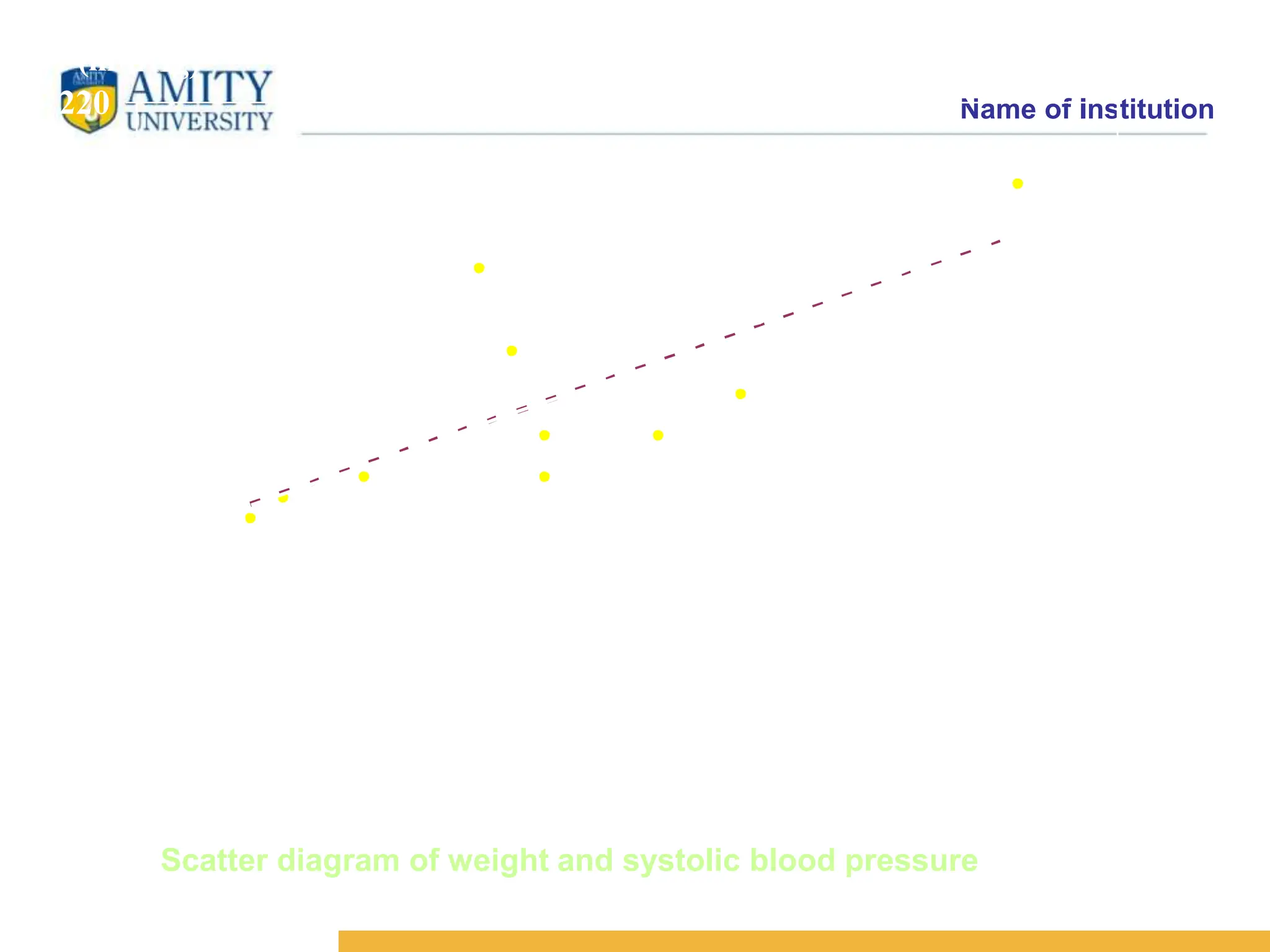
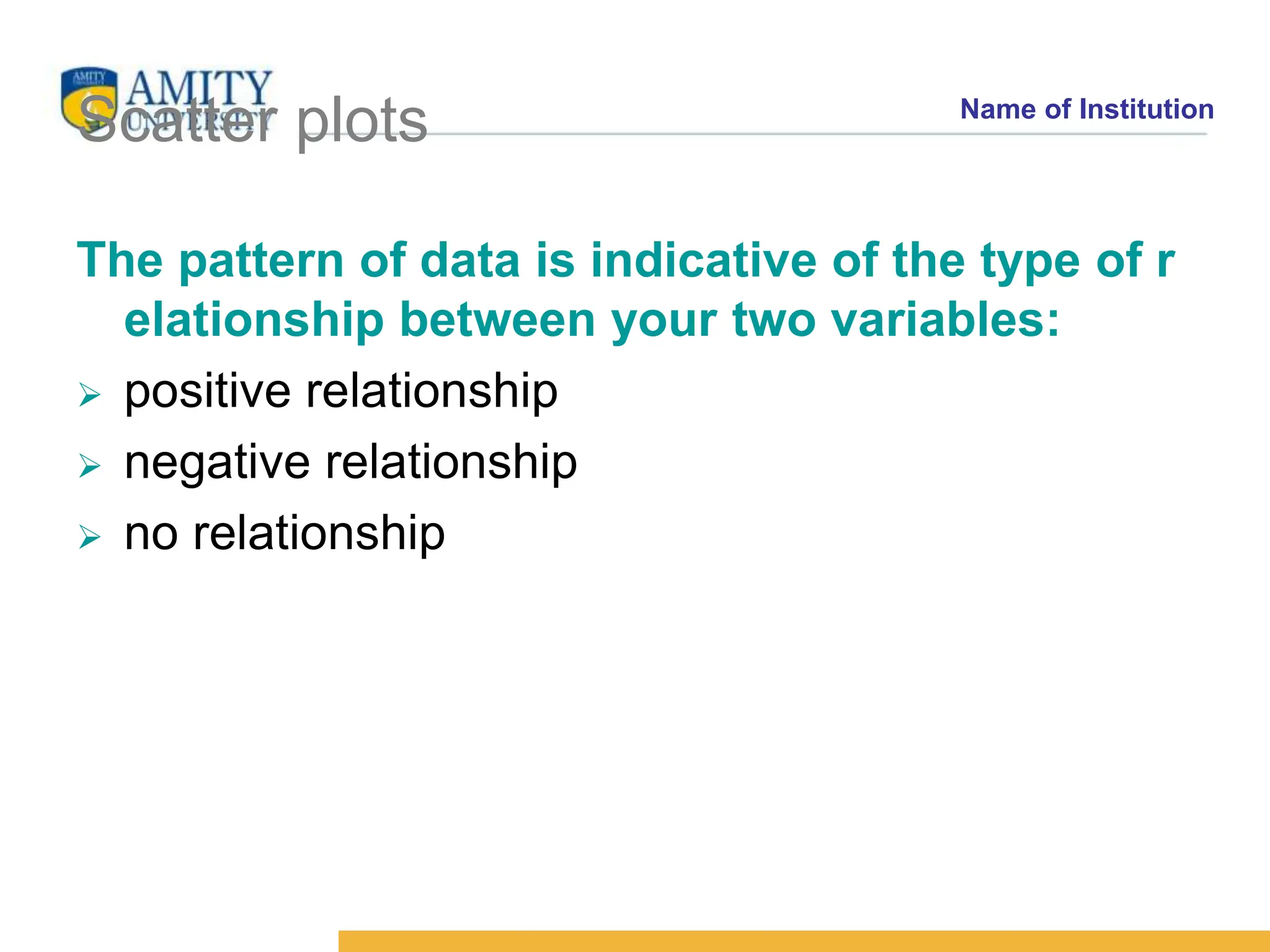
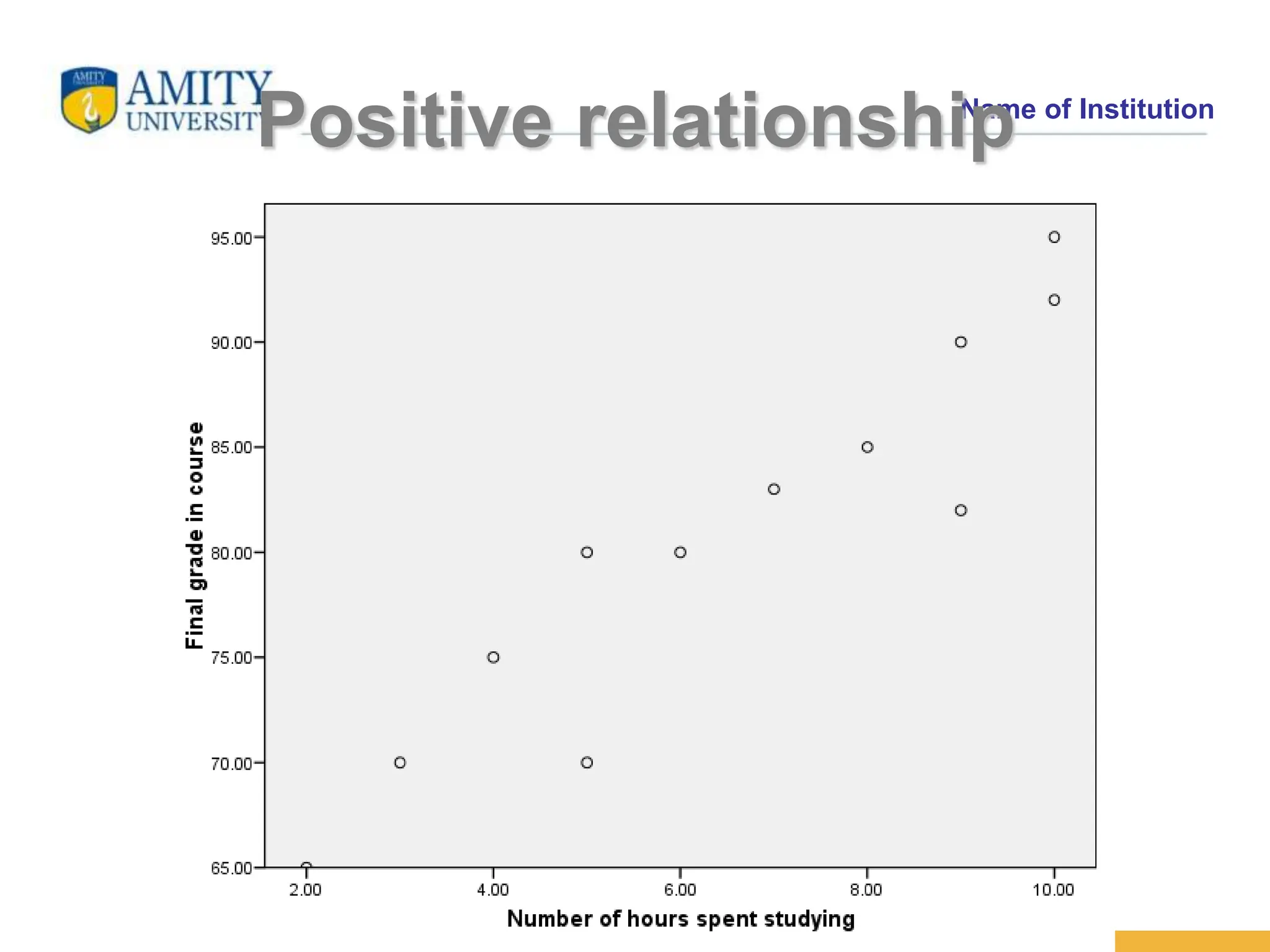
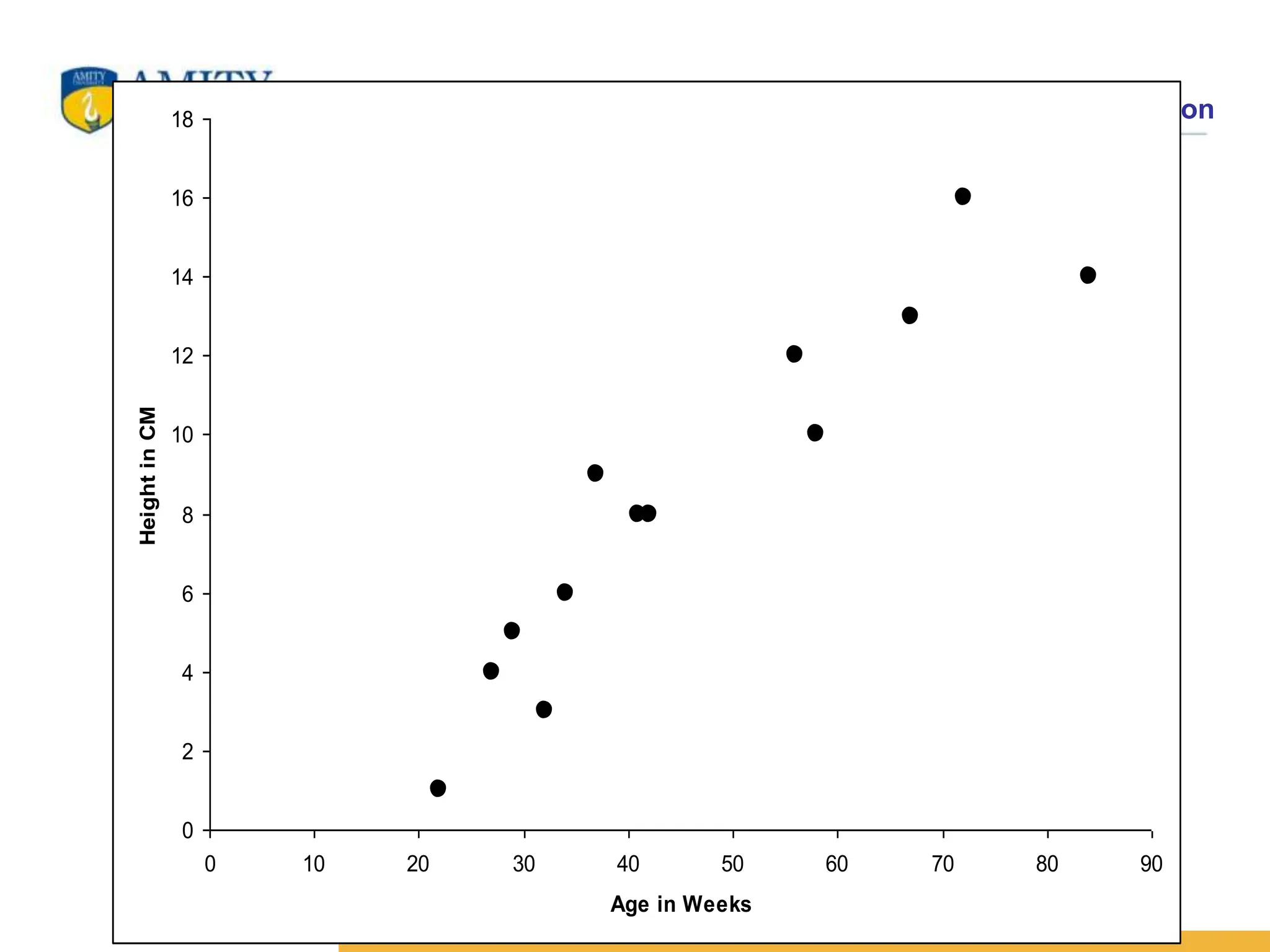
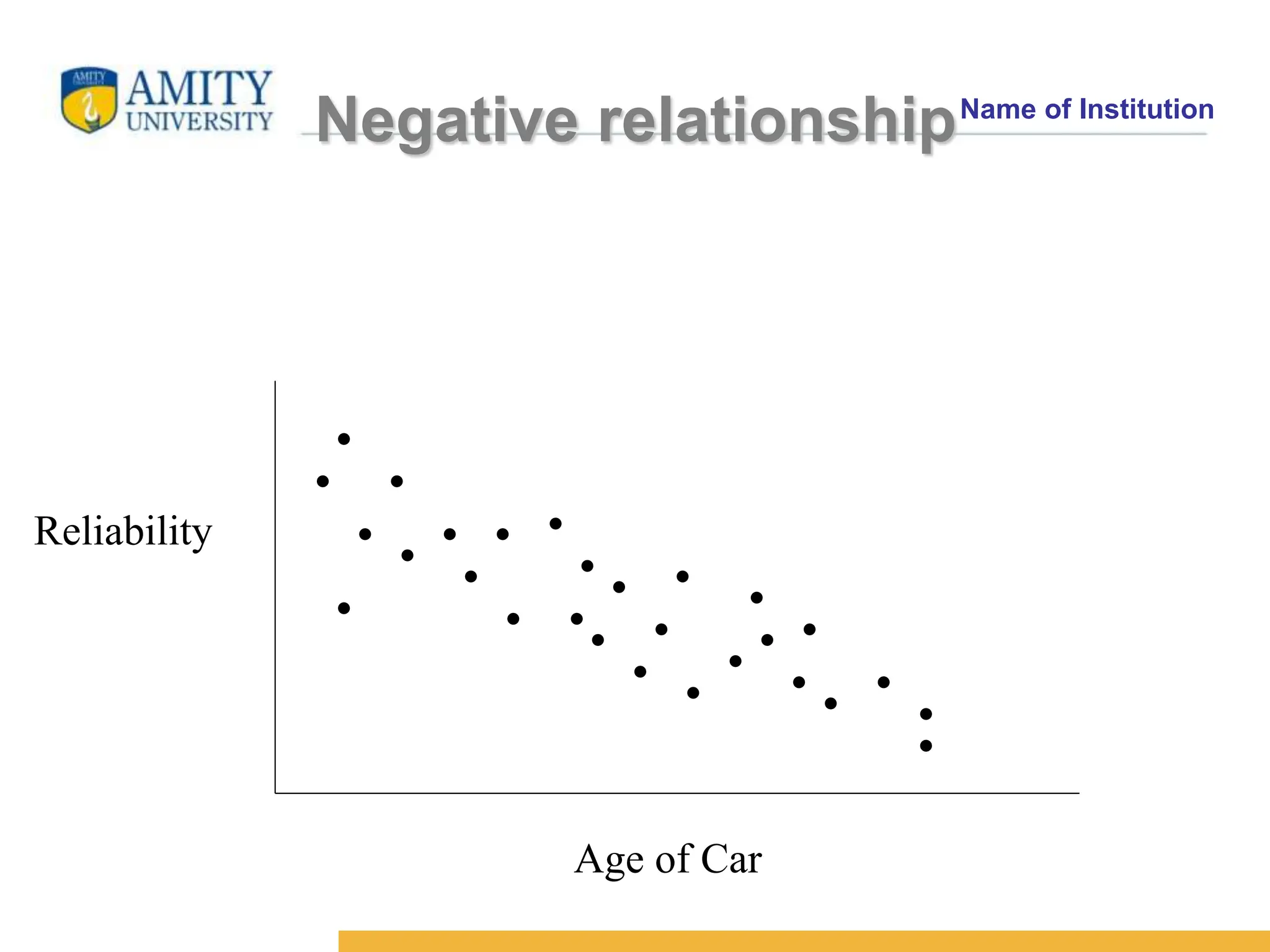
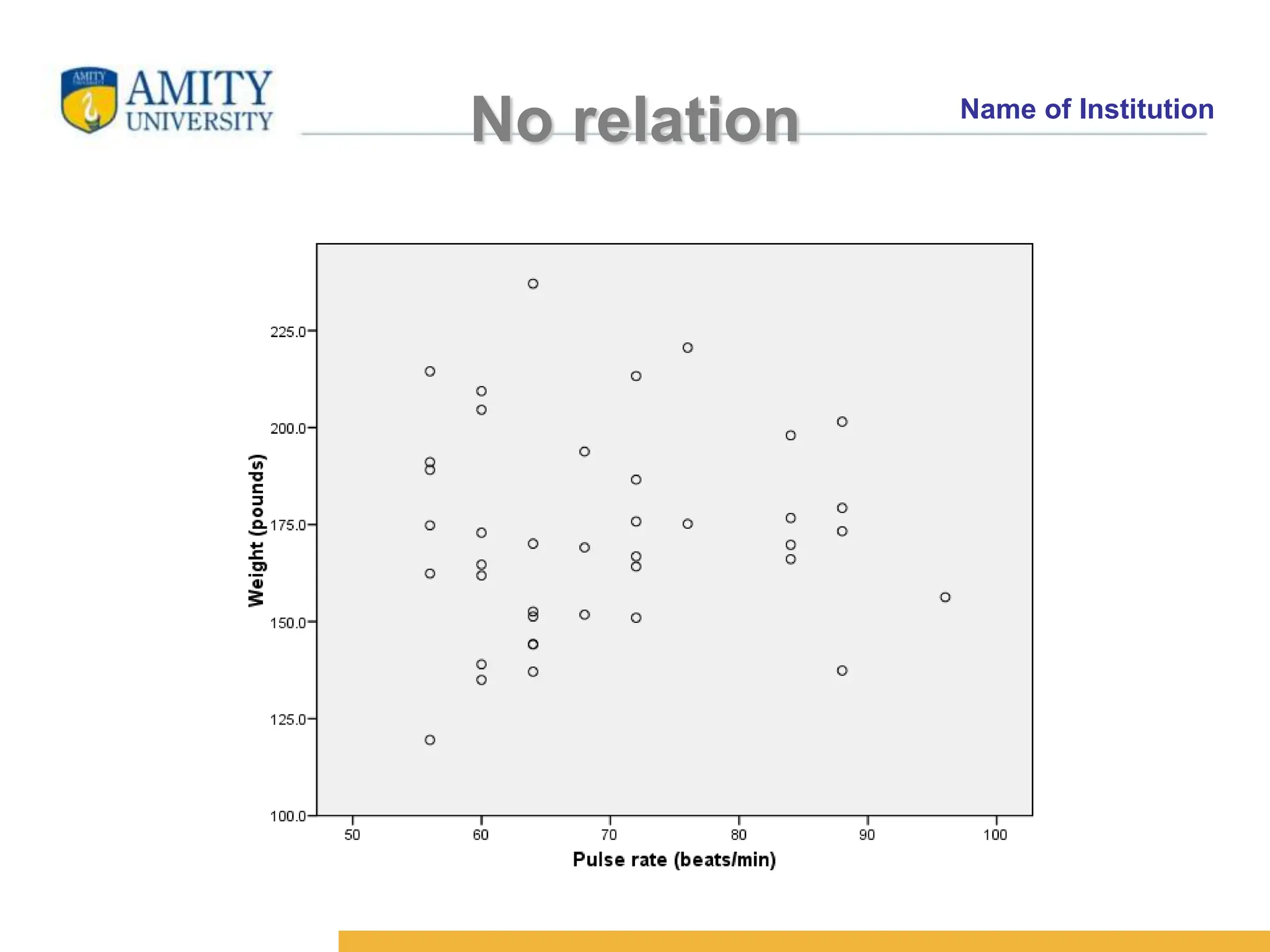
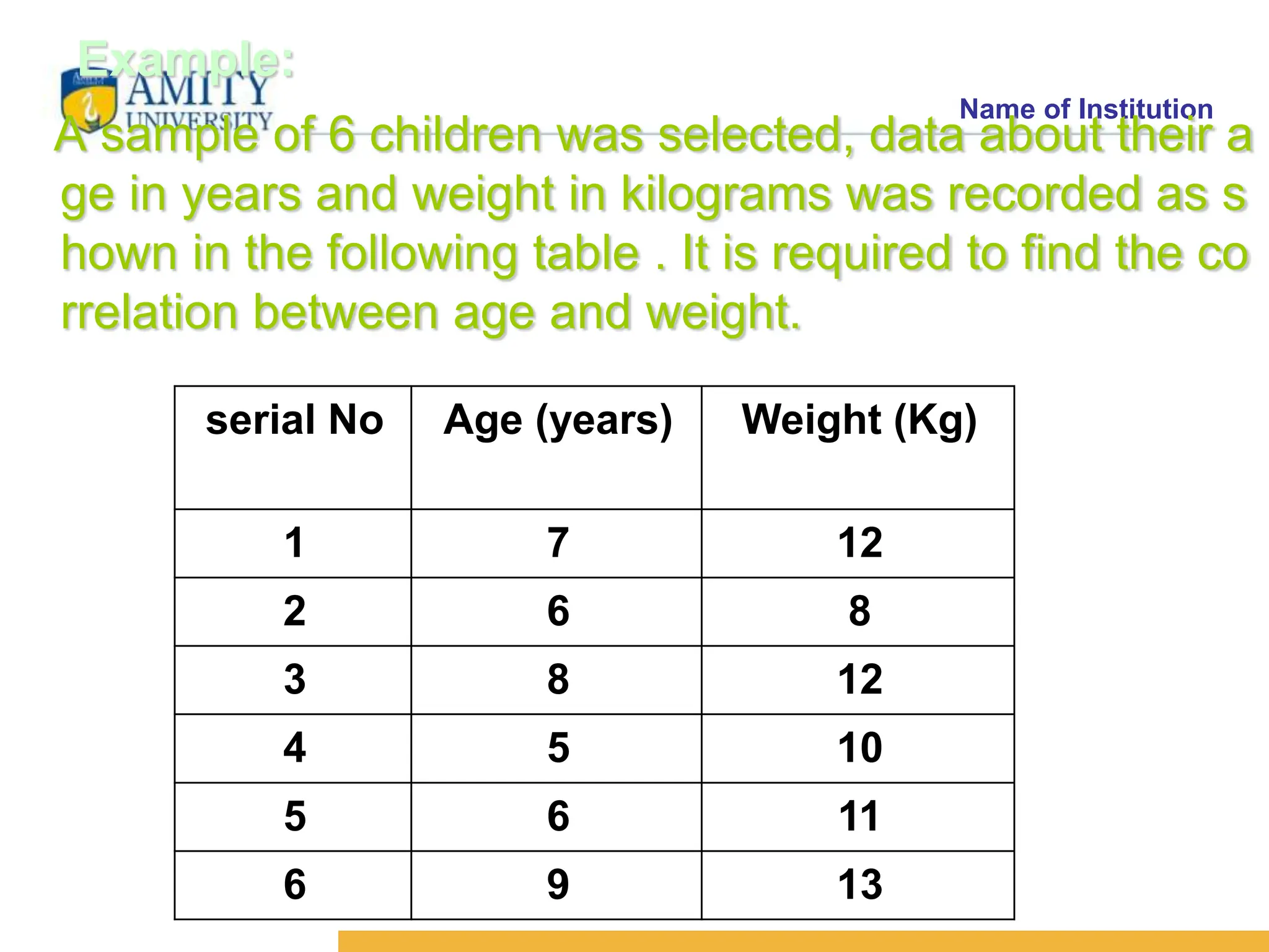
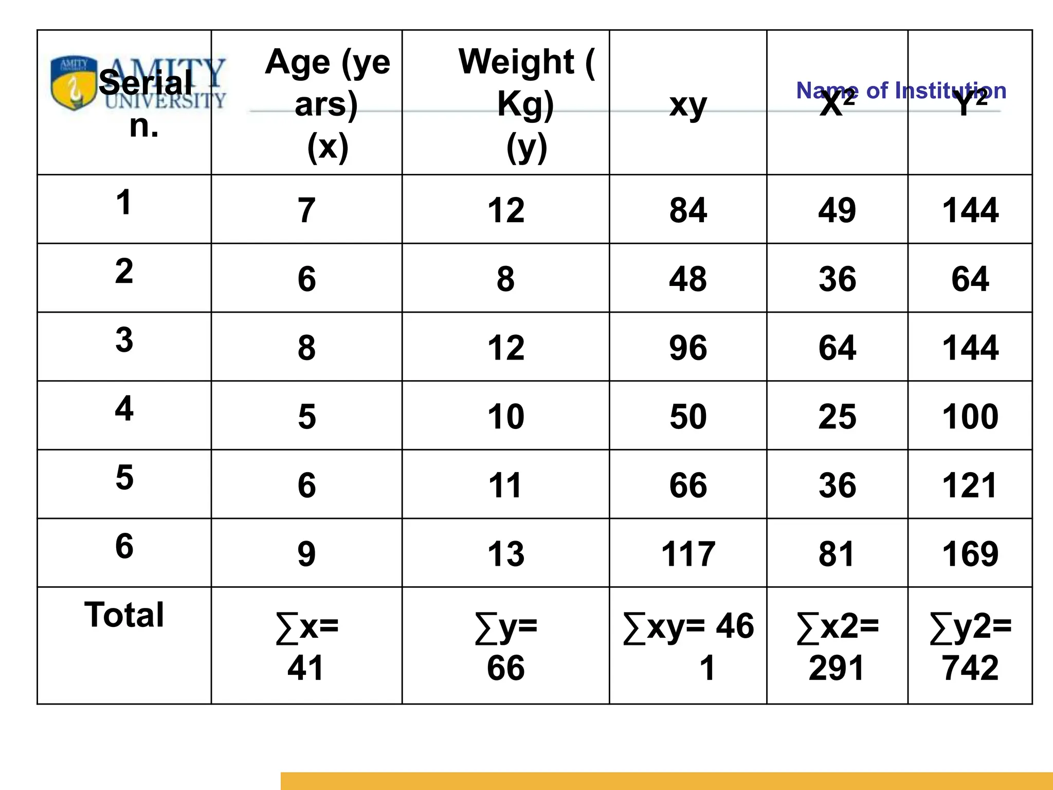
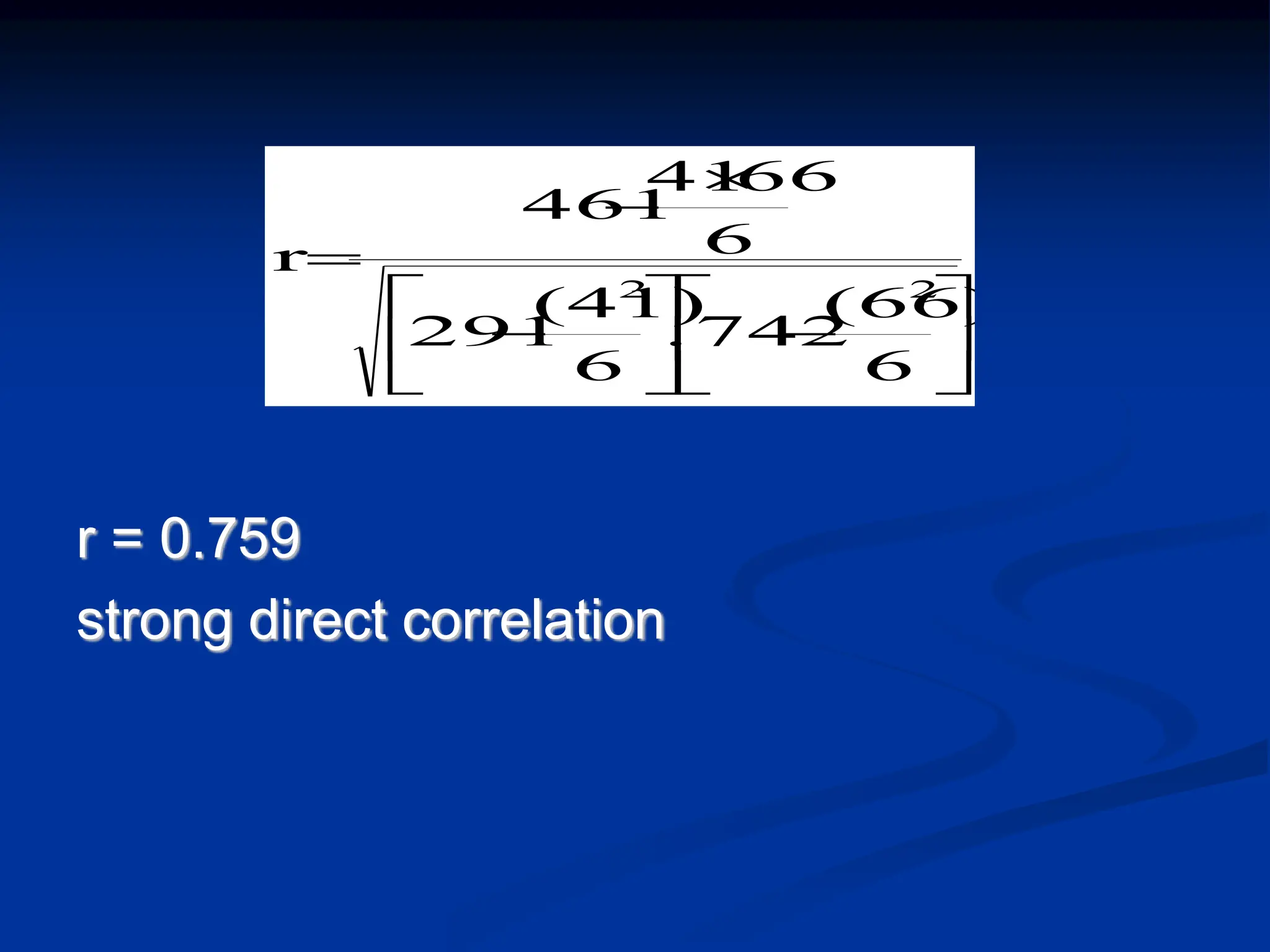
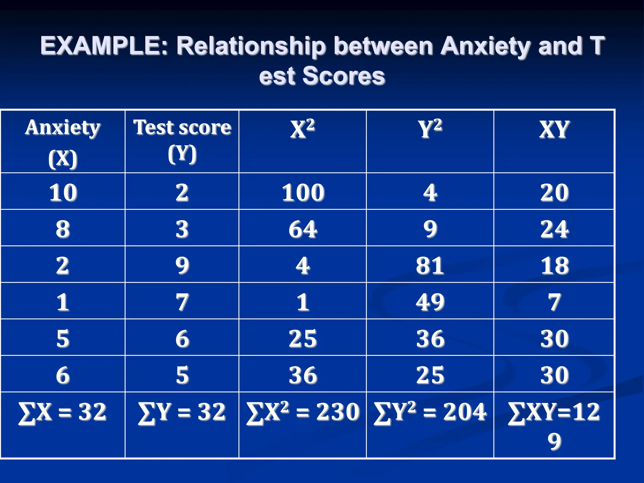
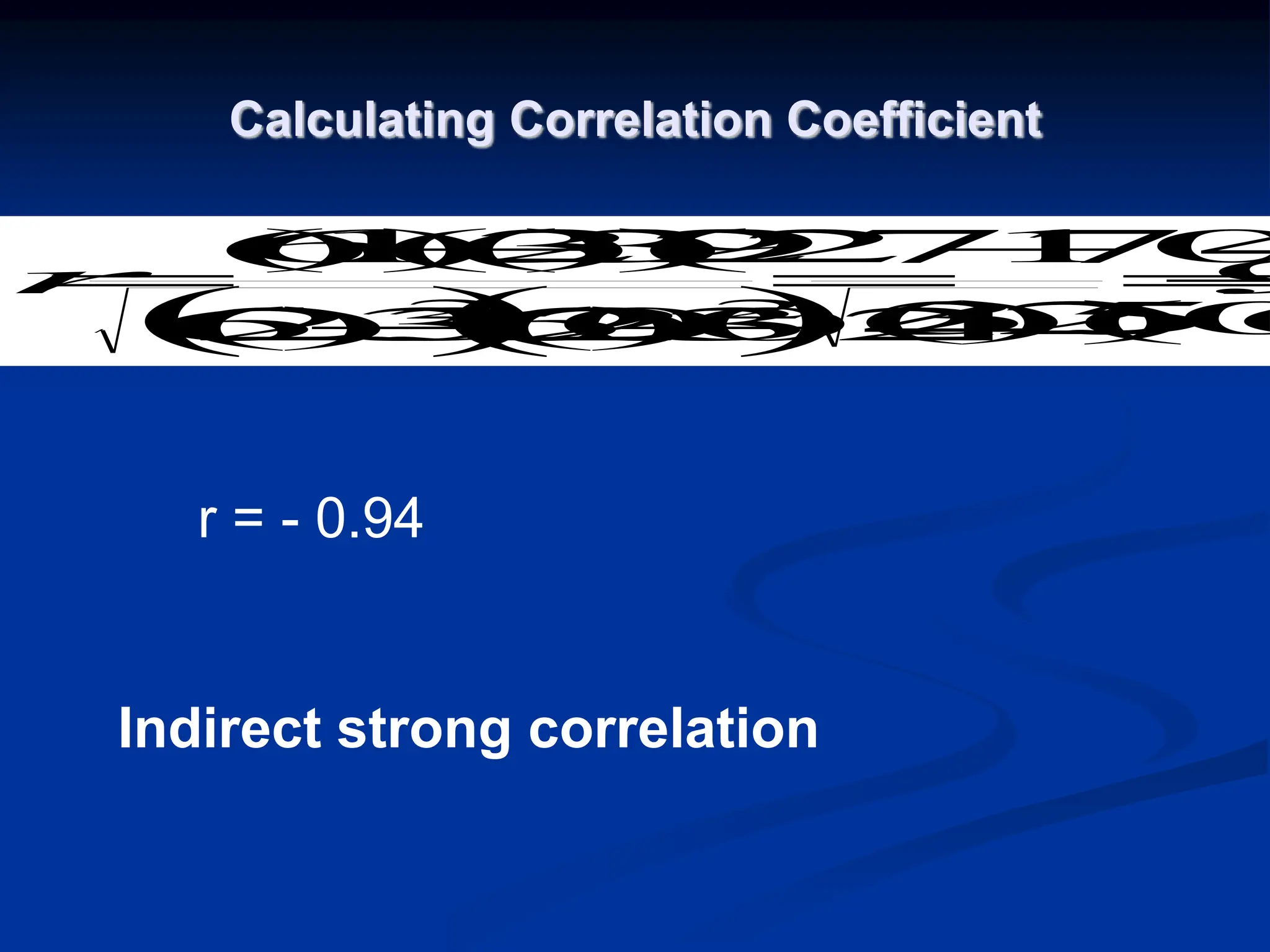
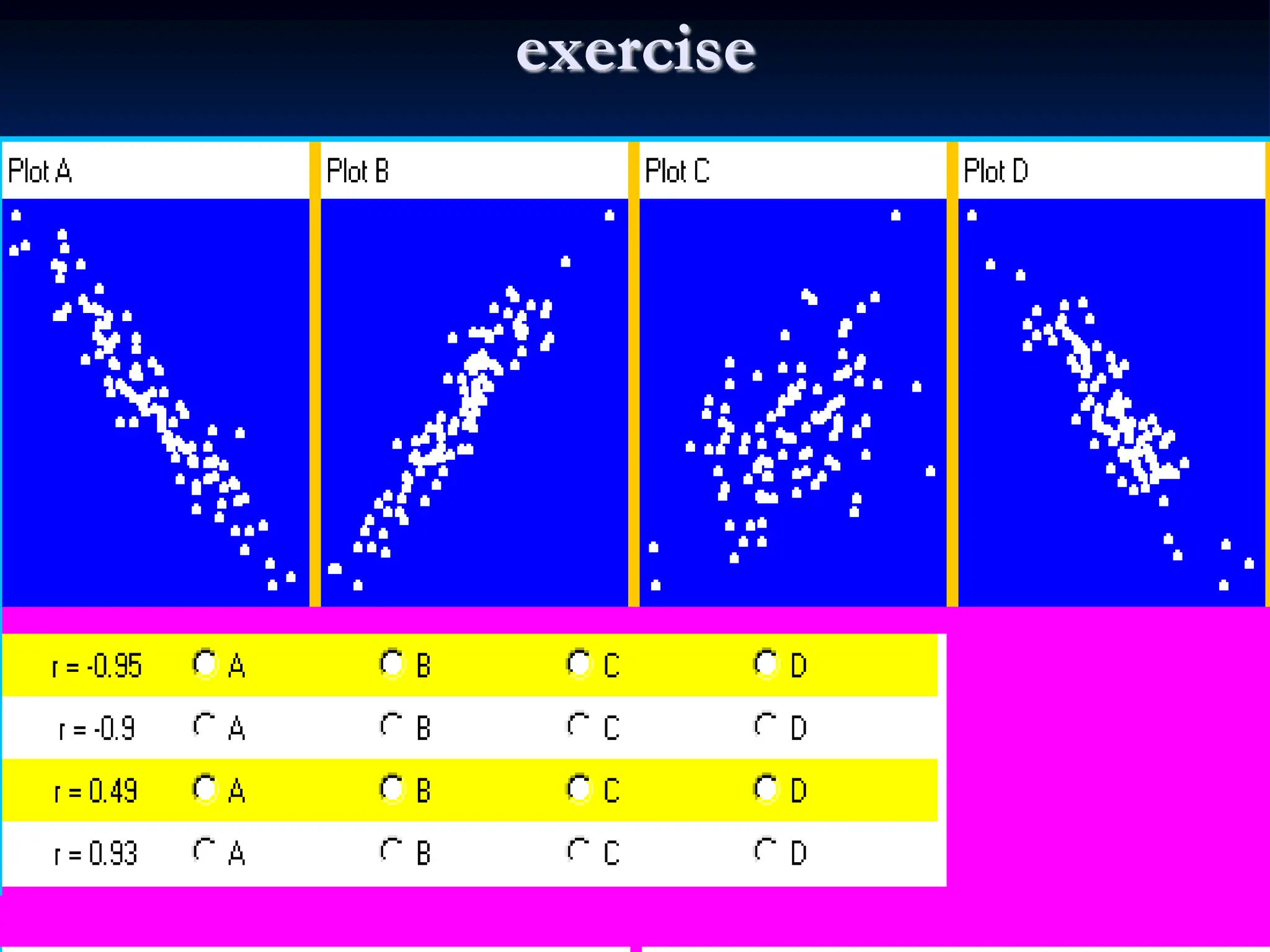
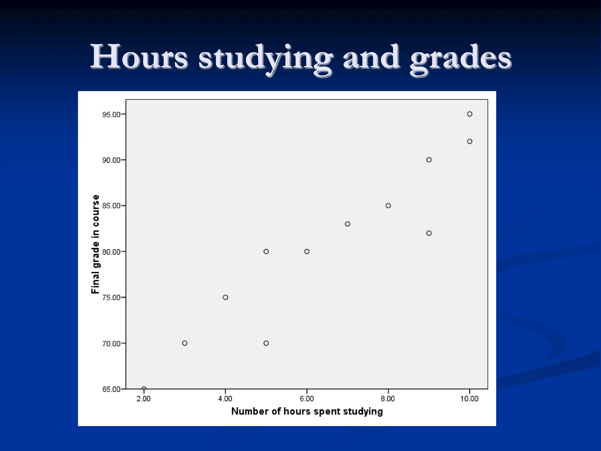
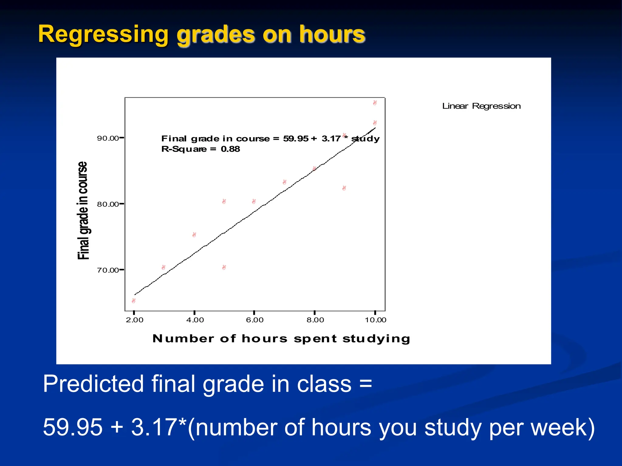
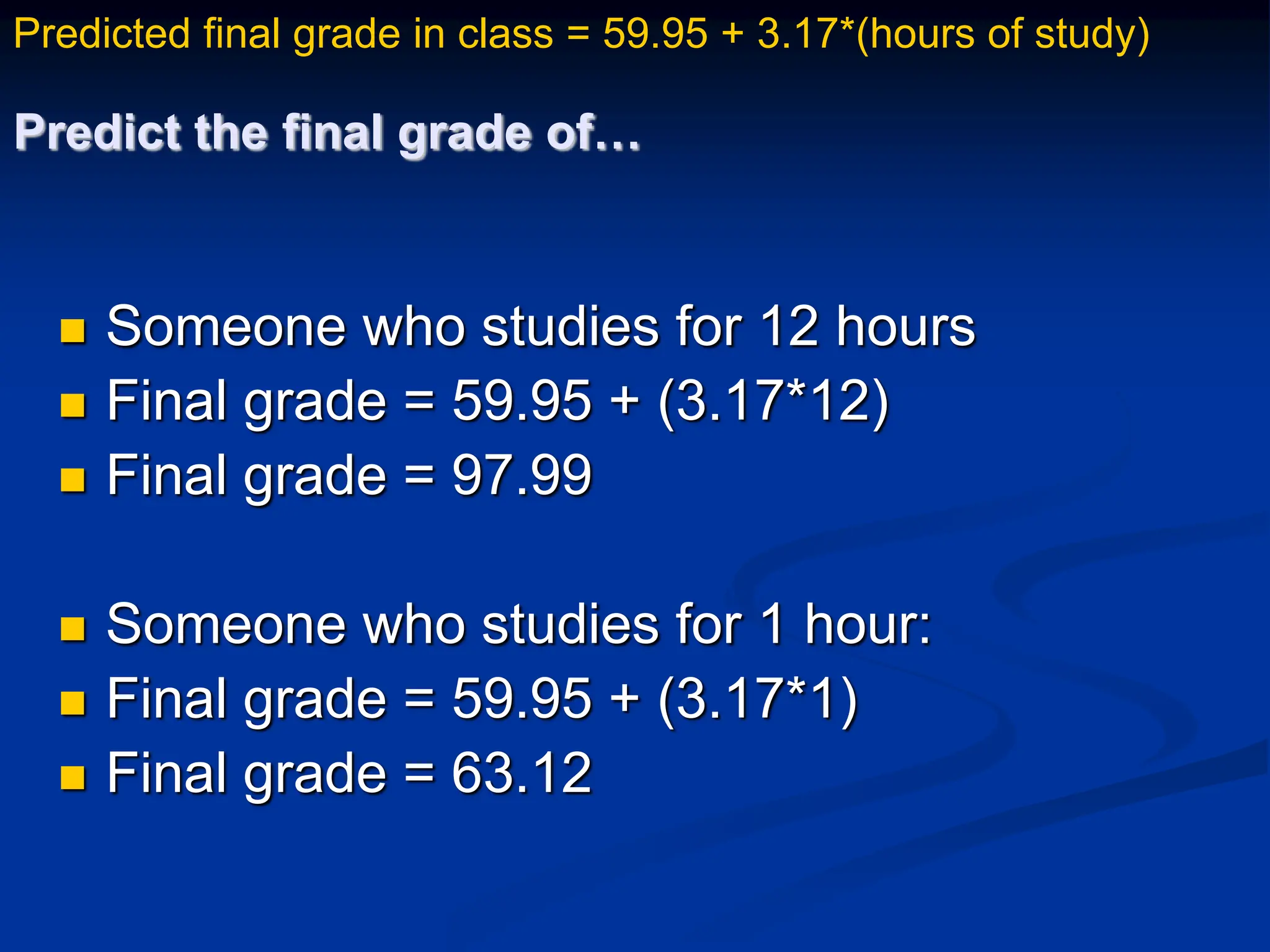
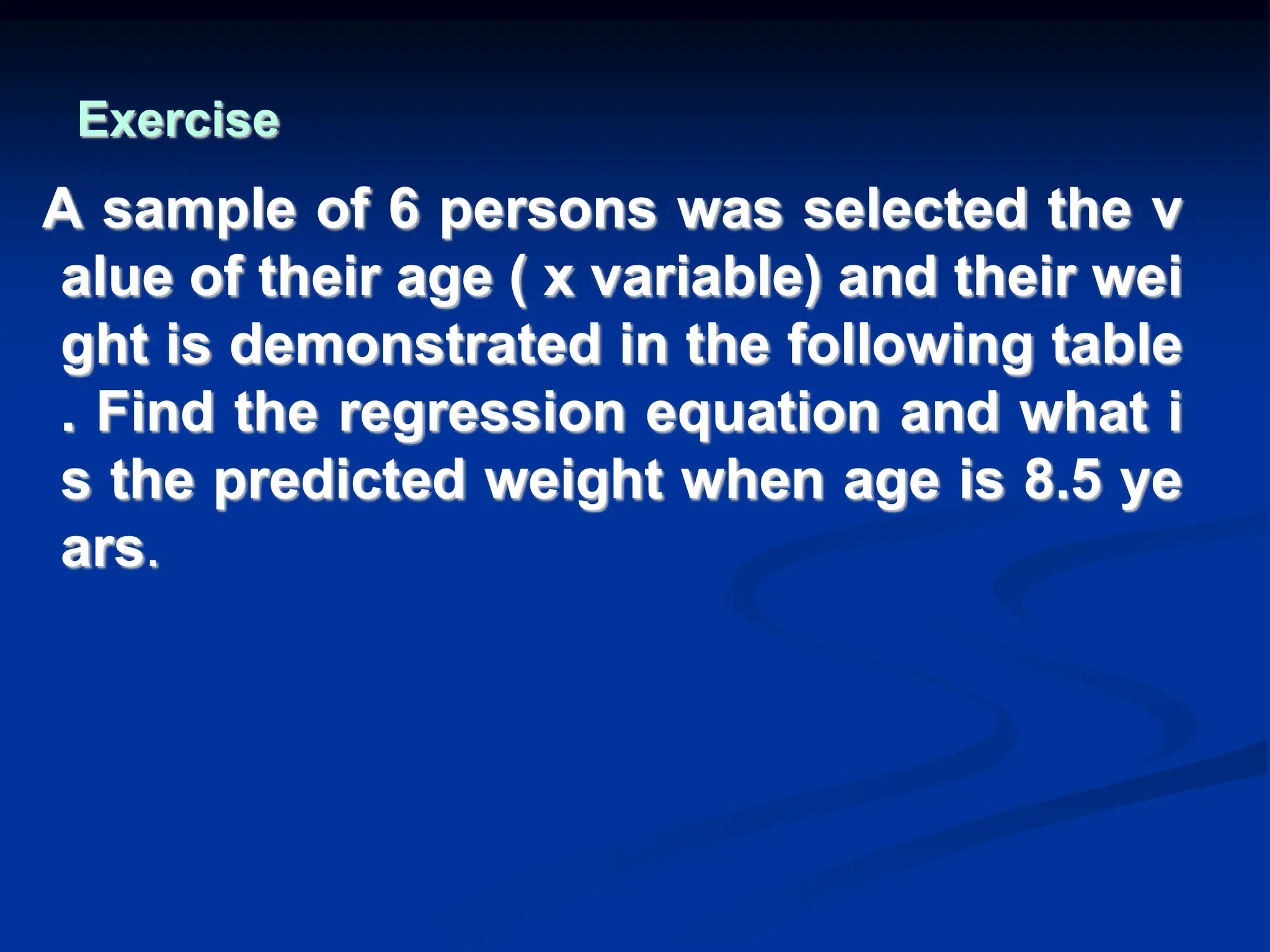
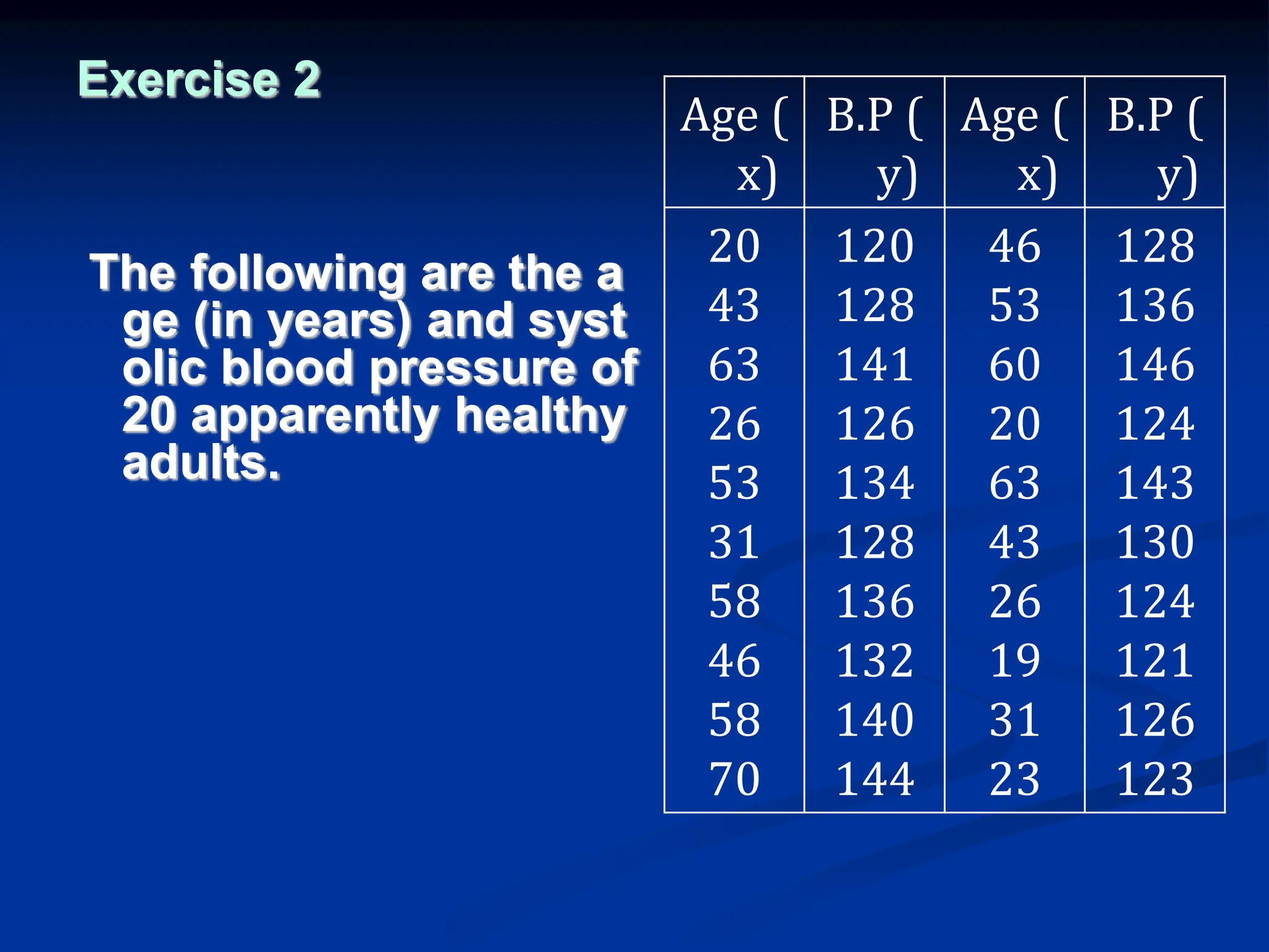
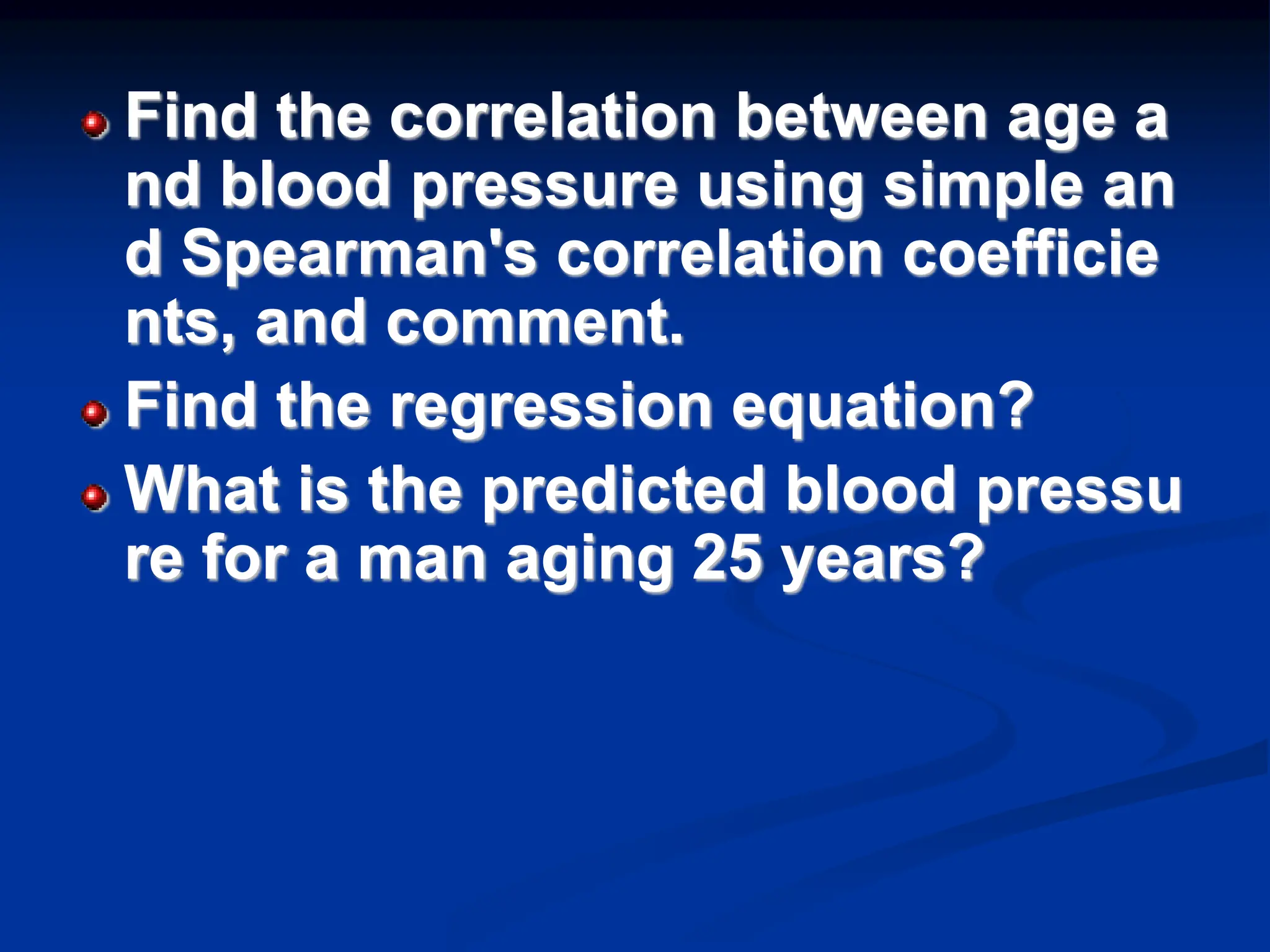
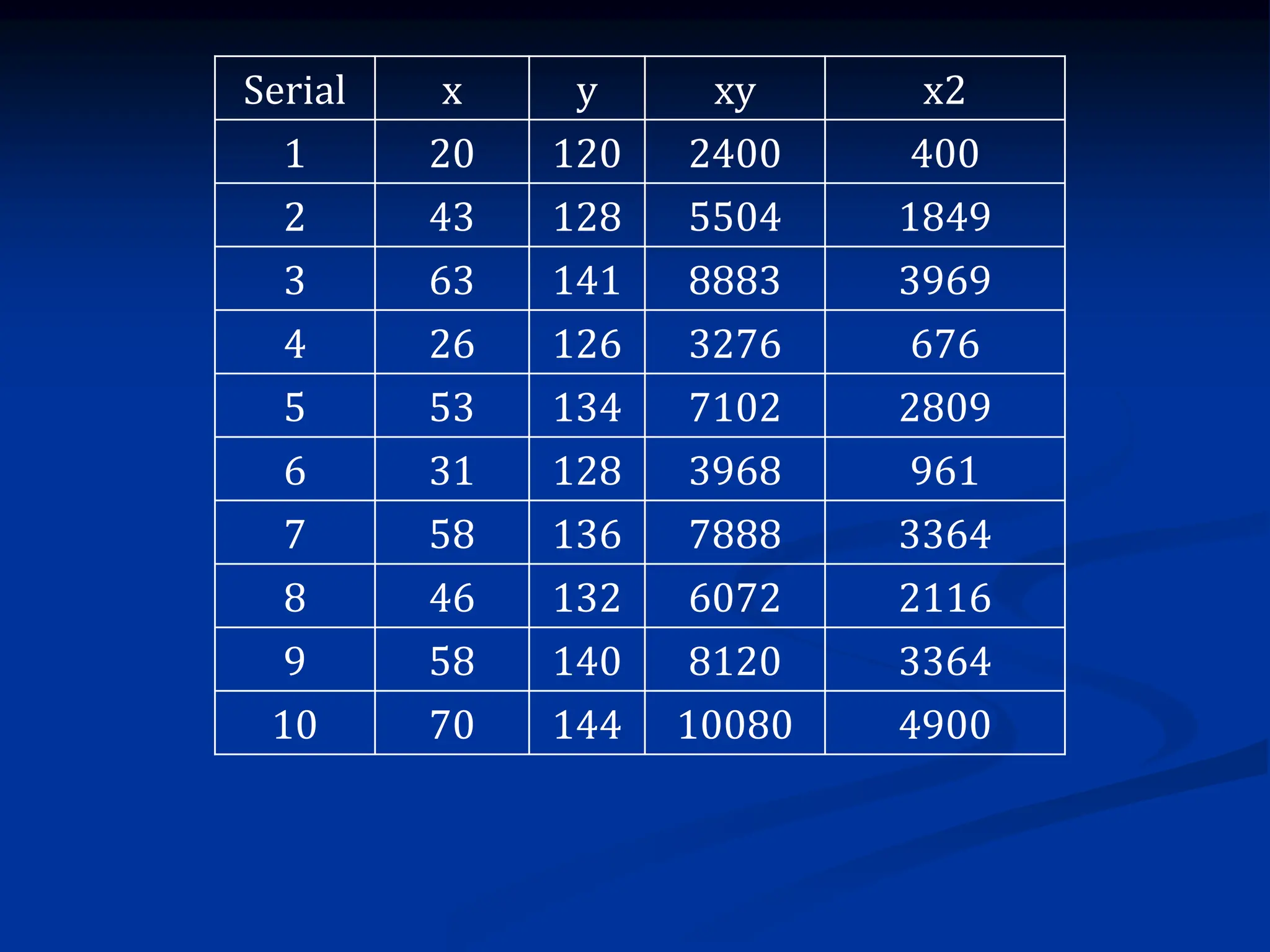
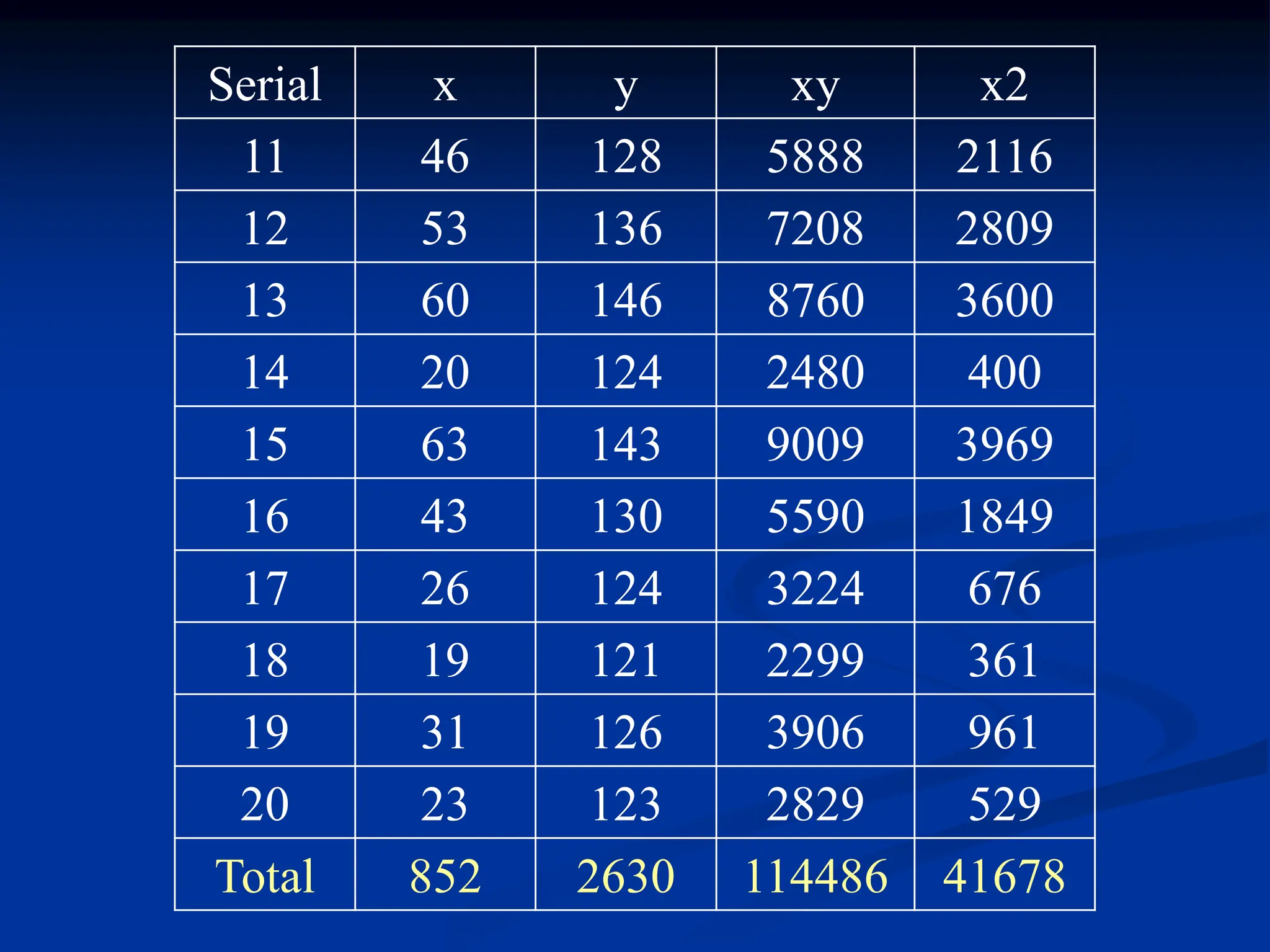
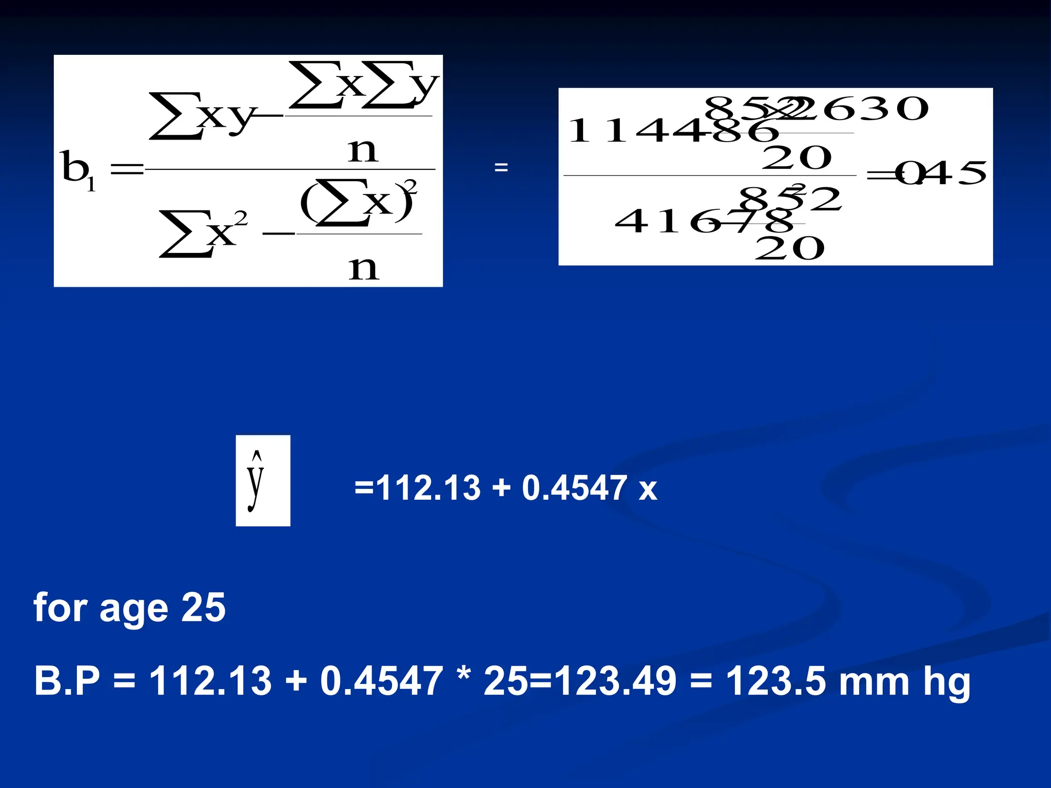
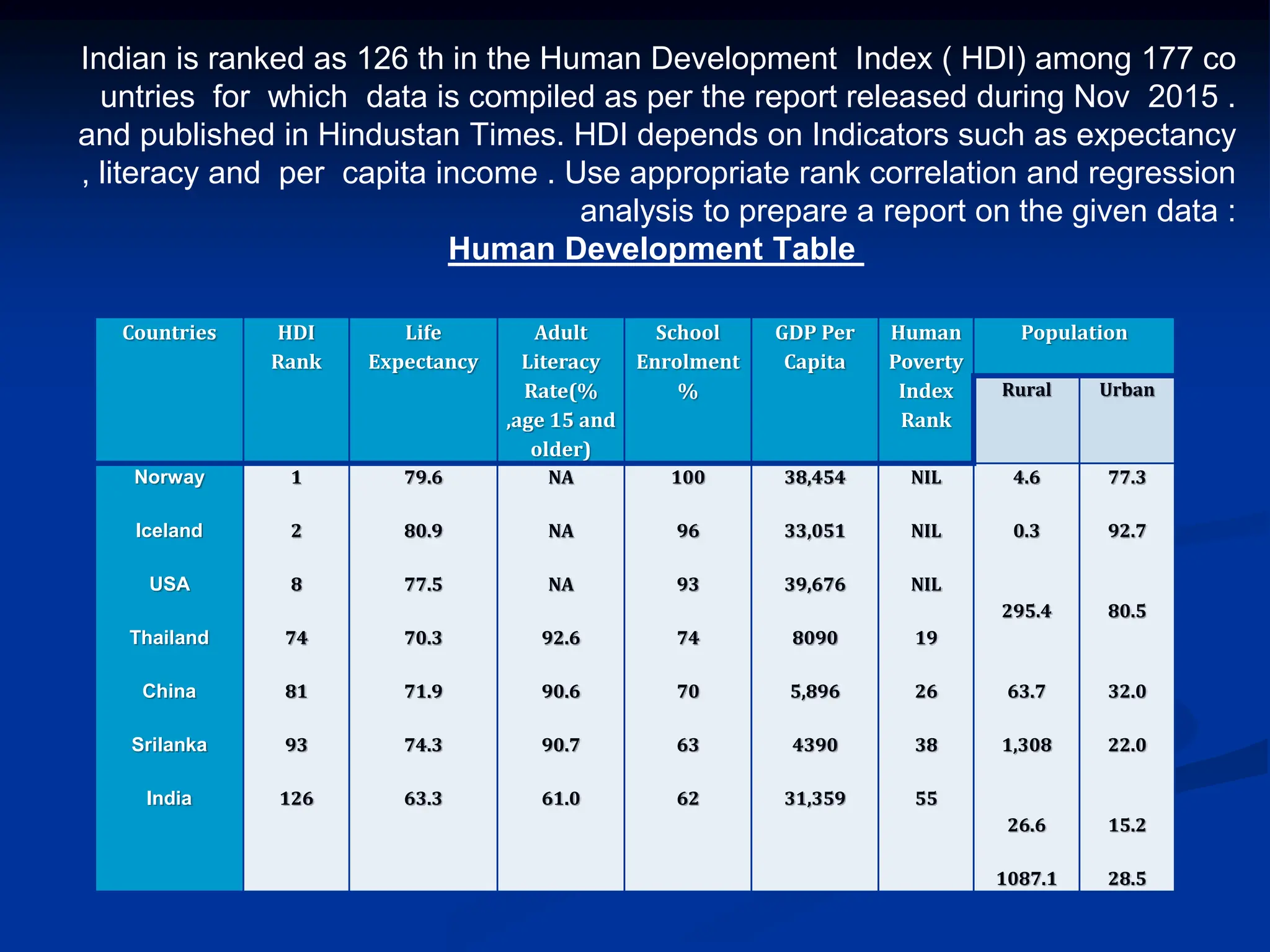
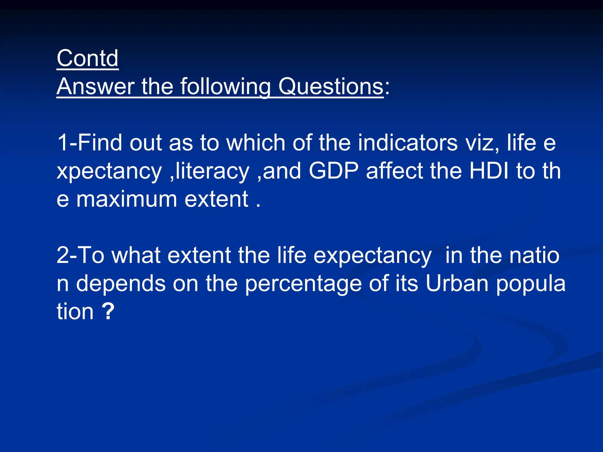
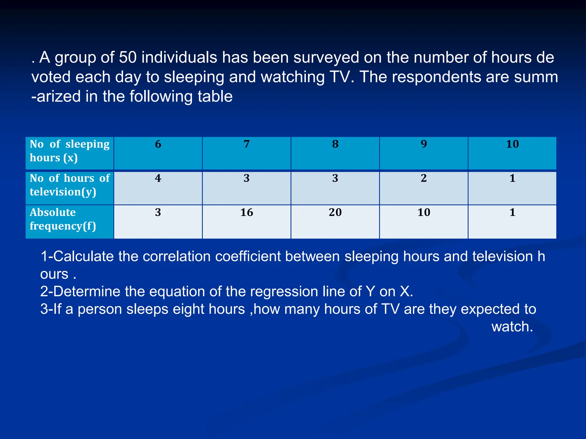
Name of Institution
Amity School of Business
BBA, ODD
Business Statistics
Dr.Neelu Tiwari
1
Name of Institution
Correlation & Regression
Dr. Neelu Tiwari
Name of Institution
Correlation
Finding the relationship between two quantit
ative variables without being able to infer c
ausal relationships
Correlation is a statistical technique used to
determine the degree to which two variabl
es are related
Name of Institution
• Rectangular coordinate
• Two quantitative variables
• One variable is called independent (X) and t
he second is called dependent (Y)
• Points are not joined
• No frequency table
Scatter diagram
Y
* *
*
X
Name of Institution
Wt.
(kg)
67 69 85 83 74 81 97 92 114 85
SBP
(mmHg)
120 125 140 160 130 180 150 140 200 130
Example
Name of Institution
Scatter diagram of weight and systolic blood press
ure
80
100
120
140
160
180
200
220
60 70 80 90 100 110 120
wt (kg)
SBP(mmHg)
Wt.
(kg)
67 69 85 83 74 81 97 92 114 85
SBP
(mmHg)
120 125 140 160 130 180 150 140 200 130
Name of Institution
80
100
120
140
160
180
200
220
60 70 80 90 100 110 120
Wt (kg)
SBP(mmHg)
Scatter diagram of weight and systolic blood pressure
Name of Institution
Scatter plots
The pattern of data is indicative of the type of r
elationship between your two variables:
 positive relationship
 negative relationship
 no relationship
Name of Institution
Positive relationship
Name of Institution
0
2
4
6
8
10
12
14
16
18
0 10 20 30 40 50 60 70 80 90
Age in Weeks
Height
in
CM
Name of Institution
11
Name of Institution
Negative relationship
Reliability
Age of Car
Name of Institution
No relation
Name of Institution
Correlation Coefficient
Statistic showing the degree of relation bet
ween two variables
Simple Correlation coefficient (r)
 It is also called Pearson's correlation
or product moment correlation
coefficient.
 It measures the nature and strength b
etween two variables of
the quantitative type.
The sign of r denotes the nature of a
ssociation
while the value of r denotes the stren
gth of association.
 If the sign is +ve this means the relation i
s direct (an increase in one variable is as
sociated with an increase in the
other variable and a decrease in one vari
able is associated with a
decrease in the other variable).
 While if the sign is -ve this means an inve
rse or indirect relationship (which means
an increase in one variable is associated
with a decrease in the other).
 The value of r ranges between ( -1) and ( +1)
 The value of r denotes the strength of the associ
ation as illustrated
by the following diagram.
-1 1
0
-0.25
-0.75 0.75
0.25
strong strong
intermediate intermediate
weak weak
no relation
perfect correlat
ion
perfect correlat
ion
Direct
indirect
If r = Zero this means no association or correlatio
n between the two variables.
If 0 < r < 0.25 = weak correlation.
If 0.25 ≤ r < 0.75 = intermediate correlation.
If 0.75 ≤ r < 1 = strong correlation.
If r = l = perfect correlation.
Name of Institution




















 
 
 

n
y)
(
y
.
n
x)
(
x
n
y
x
xy
r
2
2
2
2
How to compute the simple correlation coeffici
ent (r)
Name of Institution
Example:
A sample of 6 children was selected, data about their a
ge in years and weight in kilograms was recorded as s
hown in the following table . It is required to find the co
rrelation between age and weight.
serial No Age (years) Weight (Kg)
1 7 12
2 6 8
3 8 12
4 5 10
5 6 11
6 9 13
Name of Institution
These 2 variables are of the quantitative type, one v
ariable (Age) is called the independent and denot
ed as (X) variable and the other (weight)
is called the dependent and denoted as (Y) variab
les to find the relation between age and weight co
mpute the simple correlation coefficient using the
following formula:




















 
 
 

n
y)
(
y
.
n
x)
(
x
n
y
x
xy
r
2
2
2
2
Name of Institution
Serial
n.
Age (ye
ars)
(x)
Weight (
Kg)
(y)
xy X2 Y2
1 7 12 84 49 144
2 6 8 48 36 64
3 8 12 96 64 144
4 5 10 50 25 100
5 6 11 66 36 121
6 9 13 117 81 169
Total ∑x=
41
∑y=
66
∑xy= 46
1
∑x2=
291
∑y2=
742
r = 0.759
strong direct correlation

















6
(66)
742
.
6
(41)
291
6
66
41
461
r
2
2
EXAMPLE: Relationship between Anxiety and T
est Scores
Anxiety
(X)
Test score
(Y)
X2 Y2 XY
10 2 100 4 20
8 3 64 9 24
2 9 4 81 18
1 7 1 49 7
5 6 25 36 30
6 5 36 25 30
∑X = 32 ∑Y = 32 ∑X2 = 230 ∑Y2 = 204 ∑XY=12
9
Calculating Correlation Coefficient
 
 
9
.
)
20
)(
356
(
10
774
32
)
204
(
6
32
)
230
(
6
)
32
)(
32
(
)
129
)(
6
(
2
2








r
r = - 0.94
Indirect strong correlation
Spearman Rank Correlation Coefficient (r
s)
It is a non-parametric measure of correlation.
This procedure makes use of the two sets of ran
ks that may be assigned to the sample values of
x and Y.
Spearman Rank correlation coefficient could be
computed in the following cases:
Both variables are quantitative.
Both variables are qualitative ordinal.
One variable is quantitative and the other is qual
itative ordinal.
Procedure:
1. Rank the values of X from 1 to n where n
is the numbers of pairs of values of X and
Y in the sample.
2. Rank the values of Y from 1 to n.
3. Compute the value of di for each pair of o
bservation by subtracting the rank of Yi fr
om the rank of Xi
4. Square each di and compute ∑di2 which i
s the sum of the squared values.
5. Apply the following formula
1)
n(n
(di)
6
1
r 2
2
s




The value of rs denotes the magnitude a
nd nature of association giving the same int
erpretation as simple r.
Example
In a study of the relationship between level e
ducation and income the following data was
obtained. Find the relationship between them
and comment.
sample
numbers
level education
(X)
Income
(Y)
A Preparatory. 25
B Primary. 10
C University. 8
D secondary 10
E secondary 15
F illiterate 50
G University. 60
Answer:
(X) (Y)
Rank
X
Rank
Y
di di2
A Preparatory 25 5 3 2 4
B Primary. 10 6 5.5 0.5 0.25
C University. 8 1.5 7 -5.5 30.25
D secondary 10 3.5 5.5 -2 4
E secondary 15 3.5 4 -0.5 0.25
F illiterate 50 7 2 5 25
G university. 60 1.5 1 0.5 0.25
∑ di2=64
Comment:
There is an indirect weak correlation betwee
n level of education and income.
1
.
0
)
48
(
7
64
6
1 




s
r
exercise
Regression Analyses
Regression: technique concerned with predicting
some variables by knowing others
The process of predicting variable Y using varia
ble X
Regression
 Uses a variable (x) to predict some outcome vari
able (y)
 Tells you how values in y change as a function o
f changes in values of x
Correlation and Regression
 Correlation describes the strength of a linear rel
ationship between two variables
 Linear means “straight line”
 Regression tells us how to draw the straight line
described by the correlation
Regression
 Calculates the “best-fit” line for a certain set of data
The regression line makes the sum of the squares of
the residuals smaller than for any other line
Regression minimizes residuals
80
100
120
140
160
180
200
220
60 70 80 90 100 110 120
Wt (kg)
SBP(mmHg)
By using the least squares method (a procedure t
hat minimizes the vertical deviations of plotted p
oints surrounding a straight line) we are
able to construct a best fitting straight line to the
scatter diagram points and then formulate a regr
ession equation in the form of:



 



n
x)
(
x
n
y
x
xy
b 2
2
1
)
x
b(x
y
ŷ 

 b
bX
a
ŷ 

Regression Equation
 Regression equation
describes the regressi
on line mathematicall
y
 Intercept
 Slope
80
100
120
140
160
180
200
220
60 70 80 90 100 110 120
Wt (kg)
SBP(mmHg)
Linear Equations
Y
Y = bX + a
a = Y-intercept
X
Change
in Y
Change in X
b = Slope
bX
a
ŷ 

Hours studying and grades
Regressing grades on hours
Line
ar Re
gression
2.00 4.00 6.00 8.00 10.00
Number of hours spent studying
70.00
80.00
90.00
Fina
l
grad
e
in
cour
se












Final gr
ade in course = 59.95 + 3.17 * s
tudy
R-Squar
e = 0.88
Predicted final grade in class =
59.95 + 3.17*(number of hours you study per week)
Predict the final grade of…
 Someone who studies for 12 hours
 Final grade = 59.95 + (3.17*12)
 Final grade = 97.99
 Someone who studies for 1 hour:
 Final grade = 59.95 + (3.17*1)
 Final grade = 63.12
Predicted final grade in class = 59.95 + 3.17*(hours of study)
Exercise
A sample of 6 persons was selected the v
alue of their age ( x variable) and their wei
ght is demonstrated in the following table
. Find the regression equation and what i
s the predicted weight when age is 8.5 ye
ars.
Serial no. Age (x) Weight (y)
1
2
3
4
5
6
7
6
8
5
6
9
12
8
12
10
11
13
Answer
Serial no. Age (x) Weight (y) xy X2 Y2
1
2
3
4
5
6
7
6
8
5
6
9
12
8
12
10
11
13
84
48
96
50
66
117
49
36
64
25
36
81
144
64
144
100
121
169
Total 41 66 461 291 742
6.83
6
41
x 
 11
6
66


y
92
.
0
6
)
41
(
291
6
66
41
461
2





b
Regression equation
6.8
0.9(x
11
ŷ
(x) 


0.92
4.675
ŷ
(x) 

12
8.5
*
0.9
4.67
ŷ
(8.5) 


K
58
.
11
7.5
*
0.92
4.67
ŷ
(7.5) 


11.4
11.6
11.8
12
12.2
12.4
12.6
7 7.5 8 8.5 9
Age (in years)
Weight
(in
Kg)
we create a regression line by plotting two estimat
ed values for y against their X component, then ext
ending the line right and left.
Exercise 2
The following are the a
ge (in years) and syst
olic blood pressure of
20 apparently healthy
adults.
Age (
x)
B.P (
y)
Age (
x)
B.P (
y)
20
43
63
26
53
31
58
46
58
70
120
128
141
126
134
128
136
132
140
144
46
53
60
20
63
43
26
19
31
23
128
136
146
124
143
130
124
121
126
123
Find the correlation between age a
nd blood pressure using simple an
d Spearman's correlation coefficie
nts, and comment.
Find the regression equation?
What is the predicted blood pressu
re for a man aging 25 years?
Serial x y xy x2
1 20 120 2400 400
2 43 128 5504 1849
3 63 141 8883 3969
4 26 126 3276 676
5 53 134 7102 2809
6 31 128 3968 961
7 58 136 7888 3364
8 46 132 6072 2116
9 58 140 8120 3364
10 70 144 10080 4900
Serial x y xy x2
11 46 128 5888 2116
12 53 136 7208 2809
13 60 146 8760 3600
14 20 124 2480 400
15 63 143 9009 3969
16 43 130 5590 1849
17 26 124 3224 676
18 19 121 2299 361
19 31 126 3906 961
20 23 123 2829 529
Total 852 2630 114486 41678



 



n
x)
(
x
n
y
x
xy
b 2
2
1 4547
.
0
20
852
41678
20
2630
852
114486
2




=
=112.13 + 0.4547 x
for age 25
B.P = 112.13 + 0.4547 * 25=123.49 = 123.5 mm hg
ŷ
Indian is ranked as 126 th in the Human Development Index ( HDI) among 177 co
untries for which data is compiled as per the report released during Nov 2015 .
and published in Hindustan Times. HDI depends on Indicators such as expectancy
, literacy and per capita income . Use appropriate rank correlation and regression
analysis to prepare a report on the given data :
Human Development Table
Countries HDI
Rank
Life
Expectancy
Adult
Literacy
Rate(%
,age 15 and
older)
School
Enrolment
%
GDP Per
Capita
Human
Poverty
Index
Rank
Population
Rural Urban
Norway
Iceland
USA
Thailand
China
Srilanka
India
1
2
8
74
81
93
126
79.6
80.9
77.5
70.3
71.9
74.3
63.3
NA
NA
NA
92.6
90.6
90.7
61.0
100
96
93
74
70
63
62
38,454
33,051
39,676
8090
5,896
4390
31,359
NIL
NIL
NIL
19
26
38
55
4.6
0.3
295.4
63.7
1,308
26.6
1087.1
77.3
92.7
80.5
32.0
22.0
15.2
28.5
Contd
Answer the following Questions:
1-Find out as to which of the indicators viz, life e
xpectancy ,literacy ,and GDP affect the HDI to th
e maximum extent .
2-To what extent the life expectancy in the natio
n depends on the percentage of its Urban popula
tion ?
. A group of 50 individuals has been surveyed on the number of hours de
voted each day to sleeping and watching TV. The respondents are summ
-arized in the following table
No of sleeping
hours (x)
6 7 8 9 10
No of hours of
television(y)
4 3 3 2 1
Absolute
frequency(f)
3 16 20 10 1
1-Calculate the correlation coefficient between sleeping hours and television h
ours .
2-Determine the equation of the regression line of Y on X.
3-If a person sleeps eight hours ,how many hours of TV are they expected to
watch.
Multiple Regression
Multiple regression analysis is a straightforw
ard extension of simple regression analysi
s which allows more than one independent
variable.
 Beri,G.C.(2016).Business Statistics (3rd ed.)India :McGraw
Hill Education Pvt Ltd.
 Vohra ,N.D(2015).Quantitative Techniques in Management(
4th ed.)India: McGraw Hill Education Pvt Ltd.
 Vohra ,N.D(2013).Business Statistics (Ist ed.)India: McGra
w Hill Education Pvt Ltd.
 Sharma,J.K(2009).Business Statistics (2nd ed.) India :Pearso
n Education Pvt Ltd.

4_Correlation and and Regression (1).pptx

  • 1.
    Name of Institution AmitySchool of Business BBA, ODD Business Statistics Dr.Neelu Tiwari 1
  • 2.
    Name of Institution Correlation& Regression Dr. Neelu Tiwari
  • 3.
    Name of Institution Correlation Findingthe relationship between two quantit ative variables without being able to infer c ausal relationships Correlation is a statistical technique used to determine the degree to which two variabl es are related
  • 4.
    Name of Institution •Rectangular coordinate • Two quantitative variables • One variable is called independent (X) and t he second is called dependent (Y) • Points are not joined • No frequency table Scatter diagram Y * * * X
  • 5.
    Name of Institution Wt. (kg) 6769 85 83 74 81 97 92 114 85 SBP (mmHg) 120 125 140 160 130 180 150 140 200 130 Example
  • 6.
    Name of Institution Scatterdiagram of weight and systolic blood press ure 80 100 120 140 160 180 200 220 60 70 80 90 100 110 120 wt (kg) SBP(mmHg) Wt. (kg) 67 69 85 83 74 81 97 92 114 85 SBP (mmHg) 120 125 140 160 130 180 150 140 200 130
  • 7.
    Name of Institution 80 100 120 140 160 180 200 220 6070 80 90 100 110 120 Wt (kg) SBP(mmHg) Scatter diagram of weight and systolic blood pressure
  • 8.
    Name of Institution Scatterplots The pattern of data is indicative of the type of r elationship between your two variables:  positive relationship  negative relationship  no relationship
  • 9.
  • 10.
    Name of Institution 0 2 4 6 8 10 12 14 16 18 010 20 30 40 50 60 70 80 90 Age in Weeks Height in CM
  • 11.
  • 12.
    Name of Institution Negativerelationship Reliability Age of Car
  • 13.
  • 14.
    Name of Institution CorrelationCoefficient Statistic showing the degree of relation bet ween two variables
  • 15.
    Simple Correlation coefficient(r)  It is also called Pearson's correlation or product moment correlation coefficient.  It measures the nature and strength b etween two variables of the quantitative type.
  • 16.
    The sign ofr denotes the nature of a ssociation while the value of r denotes the stren gth of association.
  • 17.
     If thesign is +ve this means the relation i s direct (an increase in one variable is as sociated with an increase in the other variable and a decrease in one vari able is associated with a decrease in the other variable).  While if the sign is -ve this means an inve rse or indirect relationship (which means an increase in one variable is associated with a decrease in the other).
  • 18.
     The valueof r ranges between ( -1) and ( +1)  The value of r denotes the strength of the associ ation as illustrated by the following diagram. -1 1 0 -0.25 -0.75 0.75 0.25 strong strong intermediate intermediate weak weak no relation perfect correlat ion perfect correlat ion Direct indirect
  • 19.
    If r =Zero this means no association or correlatio n between the two variables. If 0 < r < 0.25 = weak correlation. If 0.25 ≤ r < 0.75 = intermediate correlation. If 0.75 ≤ r < 1 = strong correlation. If r = l = perfect correlation.
  • 20.
    Name of Institution                           n y) ( y . n x) ( x n y x xy r 2 2 2 2 How to compute the simple correlation coeffici ent (r)
  • 21.
    Name of Institution Example: Asample of 6 children was selected, data about their a ge in years and weight in kilograms was recorded as s hown in the following table . It is required to find the co rrelation between age and weight. serial No Age (years) Weight (Kg) 1 7 12 2 6 8 3 8 12 4 5 10 5 6 11 6 9 13
  • 22.
    Name of Institution These2 variables are of the quantitative type, one v ariable (Age) is called the independent and denot ed as (X) variable and the other (weight) is called the dependent and denoted as (Y) variab les to find the relation between age and weight co mpute the simple correlation coefficient using the following formula:                            n y) ( y . n x) ( x n y x xy r 2 2 2 2
  • 23.
    Name of Institution Serial n. Age(ye ars) (x) Weight ( Kg) (y) xy X2 Y2 1 7 12 84 49 144 2 6 8 48 36 64 3 8 12 96 64 144 4 5 10 50 25 100 5 6 11 66 36 121 6 9 13 117 81 169 Total ∑x= 41 ∑y= 66 ∑xy= 46 1 ∑x2= 291 ∑y2= 742
  • 24.
    r = 0.759 strongdirect correlation                  6 (66) 742 . 6 (41) 291 6 66 41 461 r 2 2
  • 25.
    EXAMPLE: Relationship betweenAnxiety and T est Scores Anxiety (X) Test score (Y) X2 Y2 XY 10 2 100 4 20 8 3 64 9 24 2 9 4 81 18 1 7 1 49 7 5 6 25 36 30 6 5 36 25 30 ∑X = 32 ∑Y = 32 ∑X2 = 230 ∑Y2 = 204 ∑XY=12 9
  • 26.
    Calculating Correlation Coefficient    9 . ) 20 )( 356 ( 10 774 32 ) 204 ( 6 32 ) 230 ( 6 ) 32 )( 32 ( ) 129 )( 6 ( 2 2         r r = - 0.94 Indirect strong correlation
  • 27.
    Spearman Rank CorrelationCoefficient (r s) It is a non-parametric measure of correlation. This procedure makes use of the two sets of ran ks that may be assigned to the sample values of x and Y. Spearman Rank correlation coefficient could be computed in the following cases: Both variables are quantitative. Both variables are qualitative ordinal. One variable is quantitative and the other is qual itative ordinal.
  • 28.
    Procedure: 1. Rank thevalues of X from 1 to n where n is the numbers of pairs of values of X and Y in the sample. 2. Rank the values of Y from 1 to n. 3. Compute the value of di for each pair of o bservation by subtracting the rank of Yi fr om the rank of Xi 4. Square each di and compute ∑di2 which i s the sum of the squared values.
  • 29.
    5. Apply thefollowing formula 1) n(n (di) 6 1 r 2 2 s     The value of rs denotes the magnitude a nd nature of association giving the same int erpretation as simple r.
  • 30.
    Example In a studyof the relationship between level e ducation and income the following data was obtained. Find the relationship between them and comment. sample numbers level education (X) Income (Y) A Preparatory. 25 B Primary. 10 C University. 8 D secondary 10 E secondary 15 F illiterate 50 G University. 60
  • 31.
    Answer: (X) (Y) Rank X Rank Y di di2 APreparatory 25 5 3 2 4 B Primary. 10 6 5.5 0.5 0.25 C University. 8 1.5 7 -5.5 30.25 D secondary 10 3.5 5.5 -2 4 E secondary 15 3.5 4 -0.5 0.25 F illiterate 50 7 2 5 25 G university. 60 1.5 1 0.5 0.25 ∑ di2=64
  • 32.
    Comment: There is anindirect weak correlation betwee n level of education and income. 1 . 0 ) 48 ( 7 64 6 1      s r
  • 33.
  • 34.
    Regression Analyses Regression: techniqueconcerned with predicting some variables by knowing others The process of predicting variable Y using varia ble X
  • 35.
    Regression  Uses avariable (x) to predict some outcome vari able (y)  Tells you how values in y change as a function o f changes in values of x
  • 36.
    Correlation and Regression Correlation describes the strength of a linear rel ationship between two variables  Linear means “straight line”  Regression tells us how to draw the straight line described by the correlation
  • 37.
    Regression  Calculates the“best-fit” line for a certain set of data The regression line makes the sum of the squares of the residuals smaller than for any other line Regression minimizes residuals 80 100 120 140 160 180 200 220 60 70 80 90 100 110 120 Wt (kg) SBP(mmHg)
  • 38.
    By using theleast squares method (a procedure t hat minimizes the vertical deviations of plotted p oints surrounding a straight line) we are able to construct a best fitting straight line to the scatter diagram points and then formulate a regr ession equation in the form of:         n x) ( x n y x xy b 2 2 1 ) x b(x y ŷ    b bX a ŷ  
  • 39.
    Regression Equation  Regressionequation describes the regressi on line mathematicall y  Intercept  Slope 80 100 120 140 160 180 200 220 60 70 80 90 100 110 120 Wt (kg) SBP(mmHg)
  • 40.
    Linear Equations Y Y =bX + a a = Y-intercept X Change in Y Change in X b = Slope bX a ŷ  
  • 41.
  • 42.
    Regressing grades onhours Line ar Re gression 2.00 4.00 6.00 8.00 10.00 Number of hours spent studying 70.00 80.00 90.00 Fina l grad e in cour se             Final gr ade in course = 59.95 + 3.17 * s tudy R-Squar e = 0.88 Predicted final grade in class = 59.95 + 3.17*(number of hours you study per week)
  • 43.
    Predict the finalgrade of…  Someone who studies for 12 hours  Final grade = 59.95 + (3.17*12)  Final grade = 97.99  Someone who studies for 1 hour:  Final grade = 59.95 + (3.17*1)  Final grade = 63.12 Predicted final grade in class = 59.95 + 3.17*(hours of study)
  • 44.
    Exercise A sample of6 persons was selected the v alue of their age ( x variable) and their wei ght is demonstrated in the following table . Find the regression equation and what i s the predicted weight when age is 8.5 ye ars.
  • 45.
    Serial no. Age(x) Weight (y) 1 2 3 4 5 6 7 6 8 5 6 9 12 8 12 10 11 13
  • 46.
    Answer Serial no. Age(x) Weight (y) xy X2 Y2 1 2 3 4 5 6 7 6 8 5 6 9 12 8 12 10 11 13 84 48 96 50 66 117 49 36 64 25 36 81 144 64 144 100 121 169 Total 41 66 461 291 742
  • 47.
  • 48.
  • 49.
    11.4 11.6 11.8 12 12.2 12.4 12.6 7 7.5 88.5 9 Age (in years) Weight (in Kg) we create a regression line by plotting two estimat ed values for y against their X component, then ext ending the line right and left.
  • 50.
    Exercise 2 The followingare the a ge (in years) and syst olic blood pressure of 20 apparently healthy adults. Age ( x) B.P ( y) Age ( x) B.P ( y) 20 43 63 26 53 31 58 46 58 70 120 128 141 126 134 128 136 132 140 144 46 53 60 20 63 43 26 19 31 23 128 136 146 124 143 130 124 121 126 123
  • 51.
    Find the correlationbetween age a nd blood pressure using simple an d Spearman's correlation coefficie nts, and comment. Find the regression equation? What is the predicted blood pressu re for a man aging 25 years?
  • 52.
    Serial x yxy x2 1 20 120 2400 400 2 43 128 5504 1849 3 63 141 8883 3969 4 26 126 3276 676 5 53 134 7102 2809 6 31 128 3968 961 7 58 136 7888 3364 8 46 132 6072 2116 9 58 140 8120 3364 10 70 144 10080 4900
  • 53.
    Serial x yxy x2 11 46 128 5888 2116 12 53 136 7208 2809 13 60 146 8760 3600 14 20 124 2480 400 15 63 143 9009 3969 16 43 130 5590 1849 17 26 124 3224 676 18 19 121 2299 361 19 31 126 3906 961 20 23 123 2829 529 Total 852 2630 114486 41678
  • 54.
            n x) ( x n y x xy b 2 2 14547 . 0 20 852 41678 20 2630 852 114486 2     = =112.13 + 0.4547 x for age 25 B.P = 112.13 + 0.4547 * 25=123.49 = 123.5 mm hg ŷ
  • 55.
    Indian is rankedas 126 th in the Human Development Index ( HDI) among 177 co untries for which data is compiled as per the report released during Nov 2015 . and published in Hindustan Times. HDI depends on Indicators such as expectancy , literacy and per capita income . Use appropriate rank correlation and regression analysis to prepare a report on the given data : Human Development Table Countries HDI Rank Life Expectancy Adult Literacy Rate(% ,age 15 and older) School Enrolment % GDP Per Capita Human Poverty Index Rank Population Rural Urban Norway Iceland USA Thailand China Srilanka India 1 2 8 74 81 93 126 79.6 80.9 77.5 70.3 71.9 74.3 63.3 NA NA NA 92.6 90.6 90.7 61.0 100 96 93 74 70 63 62 38,454 33,051 39,676 8090 5,896 4390 31,359 NIL NIL NIL 19 26 38 55 4.6 0.3 295.4 63.7 1,308 26.6 1087.1 77.3 92.7 80.5 32.0 22.0 15.2 28.5
  • 56.
    Contd Answer the followingQuestions: 1-Find out as to which of the indicators viz, life e xpectancy ,literacy ,and GDP affect the HDI to th e maximum extent . 2-To what extent the life expectancy in the natio n depends on the percentage of its Urban popula tion ?
  • 57.
    . A groupof 50 individuals has been surveyed on the number of hours de voted each day to sleeping and watching TV. The respondents are summ -arized in the following table No of sleeping hours (x) 6 7 8 9 10 No of hours of television(y) 4 3 3 2 1 Absolute frequency(f) 3 16 20 10 1 1-Calculate the correlation coefficient between sleeping hours and television h ours . 2-Determine the equation of the regression line of Y on X. 3-If a person sleeps eight hours ,how many hours of TV are they expected to watch.
  • 58.
    Multiple Regression Multiple regressionanalysis is a straightforw ard extension of simple regression analysi s which allows more than one independent variable.
  • 60.
     Beri,G.C.(2016).Business Statistics(3rd ed.)India :McGraw Hill Education Pvt Ltd.  Vohra ,N.D(2015).Quantitative Techniques in Management( 4th ed.)India: McGraw Hill Education Pvt Ltd.  Vohra ,N.D(2013).Business Statistics (Ist ed.)India: McGra w Hill Education Pvt Ltd.  Sharma,J.K(2009).Business Statistics (2nd ed.) India :Pearso n Education Pvt Ltd.

Editor's Notes