Correlation and Regression

1. ‫الرحيم‬ ‫الرحمن‬ ‫هللا‬ ‫بسم‬

2. Correlation &
Regression
Dr. Moataza Mahmoud Abdel Wahab
Lecturer of Biostatistics
High Institute of Public Health
University of Alexandria

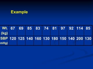
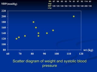
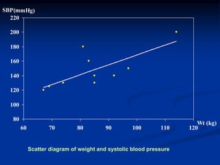
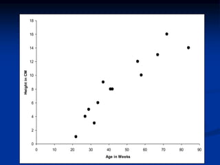
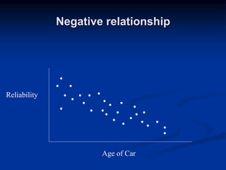
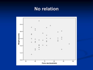
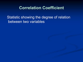
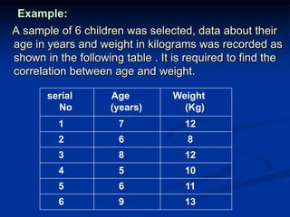
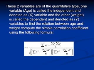
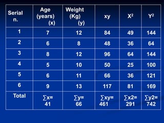
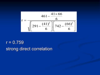
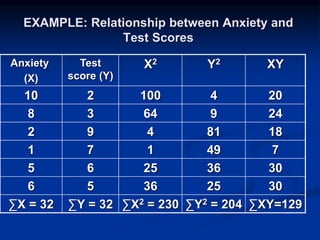
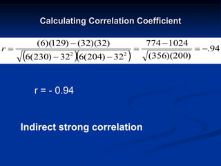
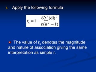
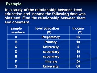
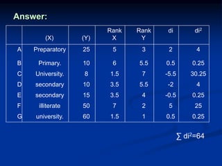
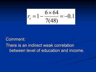
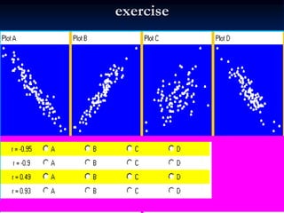
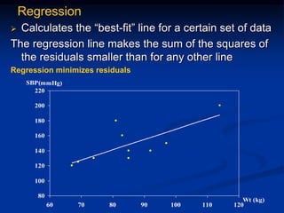
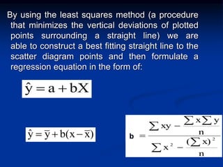
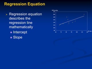
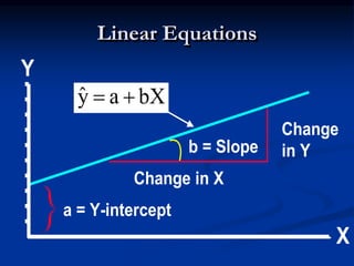
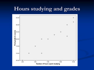
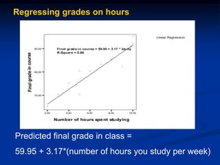
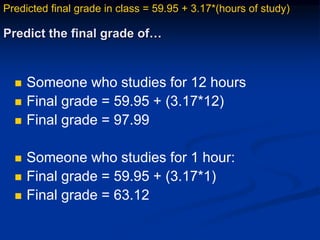
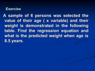
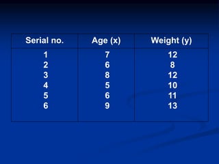
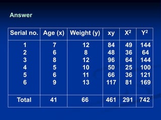
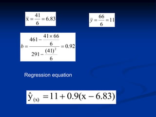
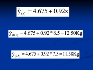
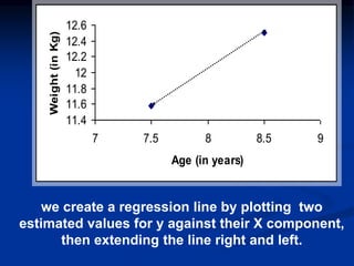
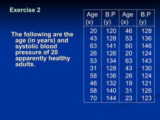
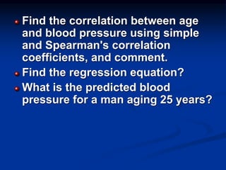
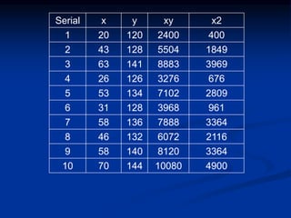
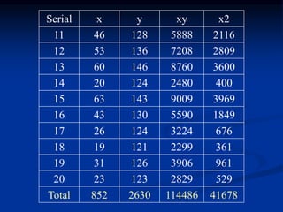
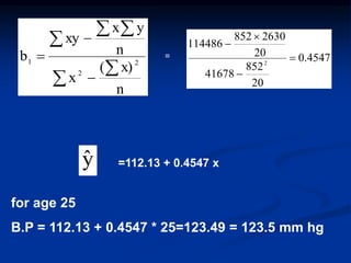
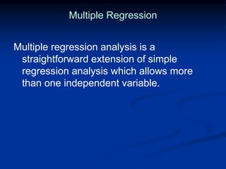
3. Correlation
Finding the relationship between two
quantitative variables without being able to
infer causal relationships
Correlation is a statistical technique used to
determine the degree to which two
variables are related

4. • Rectangular coordinate
• Two quantitative variables
• One variable is called independent (X) and
the second is called dependent (Y)
• Points are not joined
• No frequency table
Scatter diagram
Y
* *
*
X

5. Wt.
(kg)
67 69 85 83 74 81 97 92 114 85
SBP
mmHg)
120 125 140 160 130 180 150 140 200 130
Example

6. Scatter diagram of weight and systolic blood
pressure
80
100
120
140
160
180
200
220
60 70 80 90 100 110 120
wt (kg)
SBP(mmHg)
Wt.
(kg)
67 69 85 83 74 81 97 92 114 85
SBP
(mmHg)
120 125 140 160 130 180 150 140 200 130

7. 80
100
120
140
160
180
200
220
60 70 80 90 100 110 120
Wt (kg)
SBP(mmHg)
Scatter diagram of weight and systolic blood pressure

8. Scatter plots
The pattern of data is indicative of the type of
relationship between your two variables:
 positive relationship
 negative relationship
 no relationship

9. Positive relationship

10. 0
2
4
6
8
10
12
14
16
18
0 10 20 30 40 50 60 70 80 90
Age in Weeks
Height
in
CM

11. Negative relationship
Reliability
Age of Car

12. No relation

13. Correlation Coefficient
Statistic showing the degree of relation
between two variables

14. Simple Correlation coefficient (r)
 It is also called Pearson's correlation
or product moment correlation
coefficient.
 It measures the nature and strength
between two variables of
the quantitative type.

15. The sign of r denotes the nature of
association
while the value of r denotes the
strength of association.

16.  If the sign is +ve this means the relation
is direct (an increase in one variable is
associated with an increase in the
other variable and a decrease in one
variable is associated with a
decrease in the other variable).
 While if the sign is -ve this means an
inverse or indirect relationship (which
means an increase in one variable is
associated with a decrease in the other).

17.  The value of r ranges between ( -1) and ( +1)
 The value of r denotes the strength of the
association as illustrated
by the following diagram.
-1 1
0
-0.25
-0.75 0.75
0.25
strong strong
intermediate intermediate
weak weak
no relation
perfect
correlation
perfect
correlation
Direct
indirect

18. If r = Zero this means no association or
correlation between the two variables.
If 0 < r < 0.25 = weak correlation.
If 0.25 ≤ r < 0.75 = intermediate correlation.
If 0.75 ≤ r < 1 = strong correlation.
If r = l = perfect correlation.

19. 



















 
 
  
n
y)
(
y
.
n
x)
(
x
n
y
x
xy
r
2
2
2
2
How to compute the simple correlation
coefficient (r)

20. Example:
A sample of 6 children was selected, data about their
age in years and weight in kilograms was recorded as
shown in the following table . It is required to find the
correlation between age and weight.
Weight
(Kg)
Age
(years)
serial
No
12
7
1
8
6
2
12
8
3
10
5
4
11
6
5
13
9
6

21. These 2 variables are of the quantitative type, one
variable (Age) is called the independent and
denoted as (X) variable and the other (weight)
is called the dependent and denoted as (Y)
variables to find the relation between age and
weight compute the simple correlation coefficient
using the following formula:




















 
 
  
n
y)
(
y
.
n
x)
(
x
n
y
x
xy
r
2
2
2
2

22. Y2
X2
xy
Weight
(Kg)
(y)
Age
(years)
(x)
Serial
n.
144
49
84
12
7
1
64
36
48
8
6
2
144
64
96
12
8
3
100
25
50
10
5
4
121
36
66
11
6
5
169
81
117
13
9
6
∑y2=
742
∑x2=
291
∑xy=
461
∑y=
66
∑x=
41
Total

23. r = 0.759
strong direct correlation

















6
(66)
742
.
6
(41)
291
6
66
41
461
r
2
2

24. EXAMPLE: Relationship between Anxiety and
Test Scores
Anxiety
(X)
Test
score (Y)
X2 Y2 XY
10 2 100 4 20
8 3 64 9 24
2 9 4 81 18
1 7 1 49 7
5 6 25 36 30
6 5 36 25 30
∑X = 32 ∑Y = 32 ∑X2 = 230 ∑Y2 = 204 ∑XY=129

25. Calculating Correlation Coefficient
  
94
.
)
200
)(
356
(
1024
774
32
)
204
(
6
32
)
230
(
6
)
32
)(
32
(
)
129
)(
6
(
2
2








r
r = - 0.94
Indirect strong correlation

26. Spearman Rank Correlation Coefficient
(rs)
It is a non-parametric measure of correlation.
This procedure makes use of the two sets of
ranks that may be assigned to the sample
values of x and Y.
Spearman Rank correlation coefficient could be
computed in the following cases:
Both variables are quantitative.
Both variables are qualitative ordinal.
One variable is quantitative and the other is
qualitative ordinal.

27. Procedure:
1. Rank the values of X from 1 to n where n
is the numbers of pairs of values of X and
Y in the sample.
2. Rank the values of Y from 1 to n.
3. Compute the value of di for each pair of
observation by subtracting the rank of Yi
from the rank of Xi
4. Square each di and compute ∑di2 which
is the sum of the squared values.

28. 5. Apply the following formula
1)
n(n
(di)
6
1
r 2
2
s




The value of rs denotes the magnitude
and nature of association giving the same
interpretation as simple r.

29. Example
In a study of the relationship between level
education and income the following data was
obtained. Find the relationship between them
and comment.
Income
(Y)
level education
(X)
sample
numbers
25
Preparatory.
A
10
Primary.
B
8
University.
C
10
secondary
D
15
secondary
E
50
illiterate
F
60
University.
G

30. Answer:
di2
di
Rank
Y
Rank
X
(Y)
(X)
4
2
3
5
25
Preparatory
A
0.25
0.5
5.5
6
10
Primary.
B
30.25
-5.5
7
1.5
8
University.
C
4
-2
5.5
3.5
10
secondary
D
0.25
-0.5
4
3.5
15
secondary
E
25
5
2
7
50
illiterate
F
0.25
0.5
1
1.5
60
university.
G
∑ di2=64

31. Comment:
There is an indirect weak correlation
between level of education and income.
1
.
0
)
48
(
7
64
6
1 




s
r

32. exercise

33. Regression Analyses
Regression: technique concerned with predicting
some variables by knowing others
The process of predicting variable Y using
variable X

34. Regression
 Uses a variable (x) to predict some outcome
variable (y)
 Tells you how values in y change as a function
of changes in values of x

35. Correlation and Regression
 Correlation describes the strength of a linear
relationship between two variables
 Linear means “straight line”
 Regression tells us how to draw the straight line
described by the correlation

36. Regression
 Calculates the “best-fit” line for a certain set of data
The regression line makes the sum of the squares of
the residuals smaller than for any other line
Regression minimizes residuals
80
100
120
140
160
180
200
220
60 70 80 90 100 110 120
Wt (kg)
SBP(mmHg)

37. By using the least squares method (a procedure
that minimizes the vertical deviations of plotted
points surrounding a straight line) we are
able to construct a best fitting straight line to the
scatter diagram points and then formulate a
regression equation in the form of:



 



n
x)
(
x
n
y
x
xy
b 2
2
1
)
x
b(x
y
ŷ 

 b
bX
a
ŷ 


38. Regression Equation
 Regression equation
describes the
regression line
mathematically
 Intercept
 Slope
80
100
120
140
160
180
200
220
60 70 80 90 100 110 120
Wt (kg)
SBP(mmHg)

39. Linear Equations
Y
Y = bX + a
a = Y-intercept
X
Change
in Y
Change in X
b = Slope
bX
a
ŷ 


40. Hours studying and grades

41. Regressing grades on hours
Linear Regression
2.00 4.00 6.00 8.00 10.00
Number of hours spent studying
70.00
80.00
90.00
Fina
l
grad
e
in
cour
se












Final grade in course = 59.95 + 3.17 * study
R-Square = 0.88
Predicted final grade in class =
59.95 + 3.17*(number of hours you study per week)

42. Predict the final grade of…
 Someone who studies for 12 hours
 Final grade = 59.95 + (3.17*12)
 Final grade = 97.99
 Someone who studies for 1 hour:
 Final grade = 59.95 + (3.17*1)
 Final grade = 63.12
Predicted final grade in class = 59.95 + 3.17*(hours of study)

43. Exercise
A sample of 6 persons was selected the
value of their age ( x variable) and their
weight is demonstrated in the following
table. Find the regression equation and
what is the predicted weight when age is
8.5 years.

44. Weight (y)
Age (x)
Serial no.
12
8
12
10
11
13
7
6
8
5
6
9
1
2
3
4
5
6

45. Answer
Y2
X2
xy
Weight (y)
Age (x)
Serial no.
144
64
144
100
121
169
49
36
64
25
36
81
84
48
96
50
66
117
12
8
12
10
11
13
7
6
8
5
6
9
1
2
3
4
5
6
742
291
461
66
41
Total

46. 6.83
6
41
x 
 11
6
66


y
92
.
0
6
)
41
(
291
6
66
41
461
2





b
Regression equation
6.83)
0.9(x
11
ŷ(x) 



47. 0.92x
4.675
ŷ(x) 

12.50Kg
8.5
*
0.92
4.675
ŷ(8.5) 


Kg
58
.
11
7.5
*
0.92
4.675
ŷ(7.5) 



48. 11.4
11.6
11.8
12
12.2
12.4
12.6
7 7.5 8 8.5 9
Age (in years)
Weight
(in
Kg)
we create a regression line by plotting two
estimated values for y against their X component,
then extending the line right and left.

49. Exercise 2
The following are the
age (in years) and
systolic blood
pressure of 20
apparently healthy
adults.
B.P
(y)
Age
(x)
B.P
(y)
Age
(x)
128
136
146
124
143
130
124
121
126
123
46
53
60
20
63
43
26
19
31
23
120
128
141
126
134
128
136
132
140
144
20
43
63
26
53
31
58
46
58
70

50. Find the correlation between age
and blood pressure using simple
and Spearman's correlation
coefficients, and comment.
Find the regression equation?
What is the predicted blood
pressure for a man aging 25 years?

51. x2
xy
y
x
Serial
400
2400
120
20
1
1849
5504
128
43
2
3969
8883
141
63
3
676
3276
126
26
4
2809
7102
134
53
5
961
3968
128
31
6
3364
7888
136
58
7
2116
6072
132
46
8
3364
8120
140
58
9
4900
10080
144
70
10

52. x2
xy
y
x
Serial
2116
5888
128
46
11
2809
7208
136
53
12
3600
8760
146
60
13
400
2480
124
20
14
3969
9009
143
63
15
1849
5590
130
43
16
676
3224
124
26
17
361
2299
121
19
18
961
3906
126
31
19
529
2829
123
23
20
41678
114486
2630
852
Total

53. 


 



n
x)
(
x
n
y
x
xy
b 2
2
1 4547
.
0
20
852
41678
20
2630
852
114486
2




=
=112.13 + 0.4547 x
for age 25
B.P = 112.13 + 0.4547 * 25=123.49 = 123.5 mm hg
ŷ

54. Multiple Regression
Multiple regression analysis is a
straightforward extension of simple
regression analysis which allows more
than one independent variable.