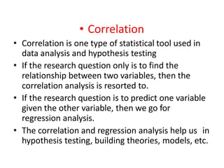
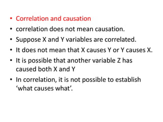
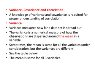
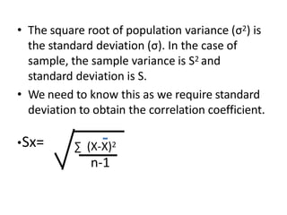
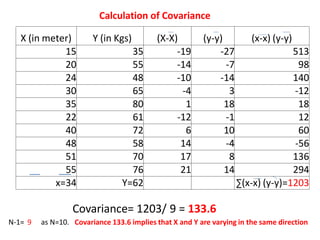
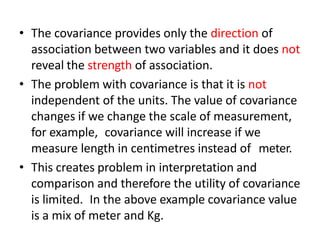
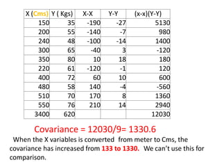
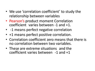
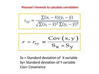
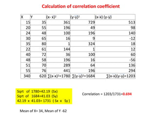
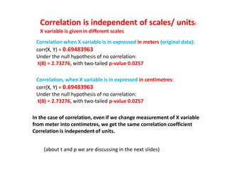
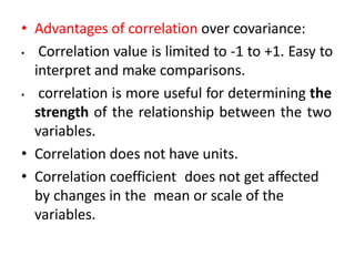
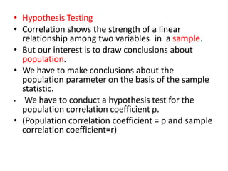
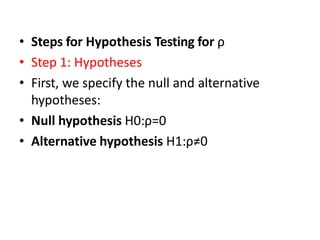
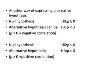
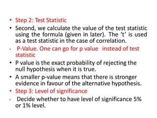
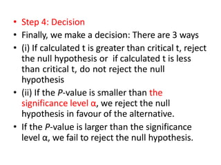
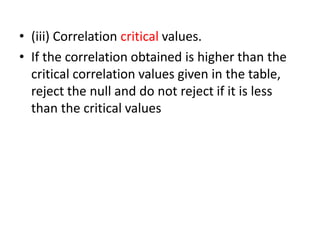
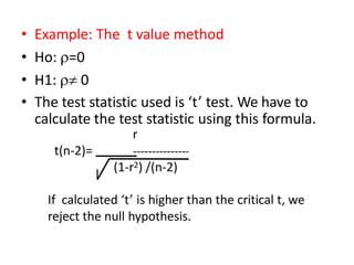
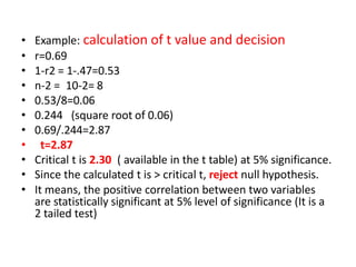
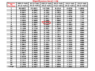
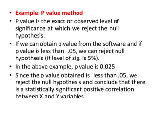
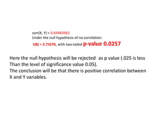
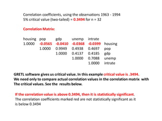
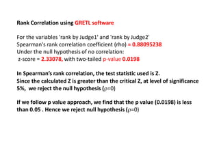
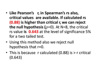
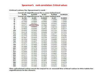
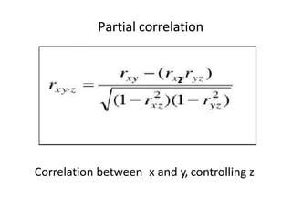
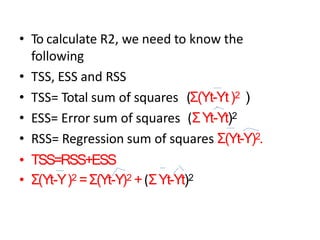
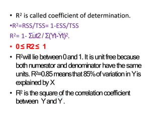
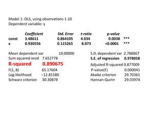
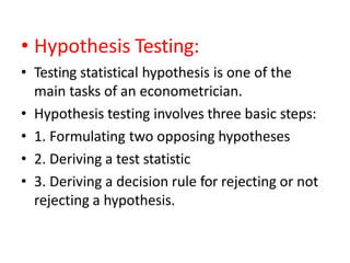
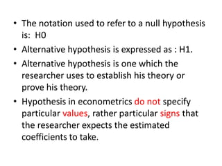
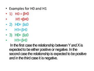
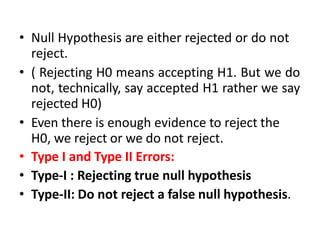
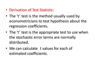
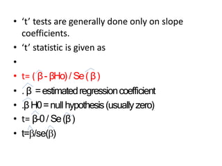
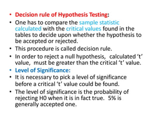
This document discusses correlation and related statistical concepts. Correlation measures the strength and direction of association between two quantitative variables. A correlation of 0 means no association, 1 means perfect positive association, and -1 means perfect negative association. Correlation is independent of measurement units and scaling of variables. Hypothesis testing is used to make inferences about the population correlation based on a sample correlation. The null hypothesis is that the population correlation is 0, and alternative hypotheses specify a non-zero correlation. The test statistic used is Student's t distribution. The null is rejected if the calculated t exceeds the critical value or if the p-value is less than the significance level.

2. • Correlation
• Correlation is one type of statistical tool used in
data analysis and hypothesis testing
• If the research question only is to find the
relationship between two variables, then the
correlation analysis is resorted to.
• If the research question is to predict one variable
given the other variable, then we go for
regression analysis.
• The correlation and regression analysis help us in
hypothesis testing, building theories, models, etc.

3. • Correlation and causation
• correlation does not mean causation.
• Suppose X and Y variables are correlated.
• It does not mean that X causes Y or Y causes X.
• It is possible that another variable Z has
caused both X and Y
• In correlation, it is not possible to establish
‘what causes what’.

4. • Variance, Covariance and Correlation
• A knowledge of variance and covariance is required for
proper understanding of correlation
• Variance
• Variance measures how far a data set is spread out.
• The variance is a numerical measure of how the
observations are dispersed around the mean in a
variable.
• Sometimes, the mean is same for all the variables under
consideration, but the variances are different.
• See the table below
• The mean is same for all 3 variables.

5. X Y Z
31 10 25
28 40 28
32 30 34
33 45 32
27 15 29
28 16 33
30 40 31
32 22 30
29 38 32
30 44 26
300 300 300
∑X/n=30 ∑X/n=30 ∑X/n= 30
The mean is same
for all variables
X, Y and Z

6. • In all above cases, the mean is same. But the
variances could be different.
• Let us see how the variances are.
• Statisticians talk about two types of variance
• Population variance (σ2 ) and sample variance
(S2).
• What is important for researchers is sample
variance as we (mostly) work with sample
data.

8. x y z (x-x)2 (y-ȳ)2 (z-z)2
31 10 25 1 400 25
28 40 28 4 100 4
32 30 34 4 0 16
33 45 32 9 225 4
27 15 29 9 225 1
28 16 33 4 196 9
30 40 31 0 100 1
32 22 30 4 64 0
29 38 32 1 64 4
30 44 26 0 196 16
∑(x-x)2=36 ∑(y-y)2=1570 ∑(z-z)2=80
Variances of x,y and z 36/9=4 1570/9=174.4 80/9=8.8
Though the mean is same (30 ) the variance is different for three series X, Y and Z.
X, Y and Z shows the marks of Economics students of 3 batches A,B and C.
Calculation of Sample Variance
X=30, Y=30 and Z=30

9. • The square root of population variance (σ2) is
the standard deviation (σ). In the case of
sample, the sample variance is S2 and
standard deviation is S.
• We need to know this as we require standard
deviation to obtain the correlation coefficient.
•Sx= ∑ (X-X)2
n-1

10. • Covariance
• The covariance measures how much two
random variables vary together.
• Covariance is similar to variance. In variance
we deal with only one variable and we study
how it varies.
• In covariance we look at two variables and try
to understand how these two variables vary
together.

11. • Covariance can be negative, positive or zero.
• If two variables move in opposite direction,
then the covariance is negative
• If two variables move in the same direction
(both variables increase or decrease), then the
covariance is positive
• The covariance is zero if two variables don’t
vary together.

12. Formula to calculate Covariance
n= the number of observations in the series (variable).
n-1 is the n adjusted for degrees of freedom

13. X (in meter) Y (in Kgs) (X-X) (y-y) (x-x) (y-y)
15 35 -19 -27 513
20 55 -14 -7 98
24 48 -10 -14 140
30 65 -4 3 -12
35 80 1 18 18
22 61 -12 -1 12
40 72 6 10 60
48 58 14 -4 -56
51 70 17 8 136
55 76 21 14 294
x=34 Y=62 ∑(x-x) (y-y)=1203
Covariance= 1203/ 9 = 133.6
as N=10. Covariance 133.6 implies that X and Y are varying in the same direction
N-1= 9
Calculation of Covariance

14. • The covariance provides only the direction of
association between two variables and it does not
reveal the strength of association.
• The problem with covariance is that it is not
independent of the units. The value of covariance
changes if we change the scale of measurement,
for example, covariance will increase if we
measure length in centimetres instead of meter.
• This creates problem in interpretation and
comparison and therefore the utility of covariance
is limited. In the above example covariance value
is a mix of meter and Kg.

15. X (Cms) Y ( Kgs) X-X Y-Y (x-x)(Y-Y)
150 35 -190 -27 5130
200 55 -140 -7 980
240 48 -100 -14 1400
300 65 -40 3 -120
350 80 10 18 180
220 61 -120 -1 120
400 72 60 10 600
480 58 140 -4 -560
510 70 170 8 1360
550 76 210 14 2940
3400 620 12030
Covariance = 12030/9= 1330.6
When the X variables is converted from meter to Cms, the
covariance has increased from 133 to 1330. We can’t use this for
comparison.

16. • Correlation
• The correlation is one of the most commonly
used statistical technique by the researchers.
• Correlation is a measure of the strength of a
linear relationship between two quantitative
variables. It also shows the direction.
• A correlation is a single number that describes
the degree of relationship between two
variables.

17. • We use ‘correlation coefficient’ to study the
relationship between variables
• Pearson’s product moment Correlation
coefficient varies between -1 and +1.
• -1 means perfect negative correlation
• +1 means perfect positive correlation.
• Correlation coefficient zero means that there is
no correlation between two variables.
• These are extreme situations and the
coefficient varies between -1 and +1

18. Sx = Standard deviation of X variable
Sy= Standard deviation of Y variable
Cov= Covariance
Pearson’s formula to calculate correlation

19. X Y (x- x)2 (y-y)2 (x-x) (y-y)
15 35 361 729 513
20 55 196 49 98
24 48 100 196 140
30 65 16 9 -12
35 80 1 324 18
22 61 144 1 12
40 72 36 100 60
48 58 196 16 -56
51 70 289 64 136
55 76 441 196 294
340 620 ∑(x-x)2=1780 ∑(y-y)2=1684 ∑(x-x)(y-y)=1203
Sqrt of 1780=42.19 (Sx)
Sqrt of 1684=41.03 (Sy)
42.19 x 41.03= 1731 ( Sx x Sy )
Correlation = 1203/1731=0.694
Calculation of correlation coefficient
Mean of X= 34, Mean of Y -62

20. Correlation is independent of scales/ units:
X variable is given in different scales
Correlation when X variable is in expressed in meters (original data):
corr(X, Y) = 0.69483963
Under the null hypothesis of no correlation:
t(8) = 2.73276, with two-tailed p-value 0.0257
Correlation, when X variable is in expressed in centimetres:
corr(X, Y) = 0.69483963
Under the null hypothesis of no correlation:
t(8) = 2.73276, with two-tailed p-value 0.0257
In the case of correlation, even if we change measurement of X variable
from meter into centimetres, we get the same correlation coefficient
Correlation is independent of units.
(about t and p we are discussing in the next slides)

21. • Advantages of correlation over covariance:
• Correlation value is limited to -1 to +1. Easy to
interpret and make comparisons.
• correlation is more useful for determining the
strength of the relationship between the two
variables.
• Correlation does not have units.
• Correlation coefficient does not get affected
by changes in the mean or scale of the
variables.

22. • Hypothesis Testing
• Correlation shows the strength of a linear
relationship among two variables in a sample.
• But our interest is to draw conclusions about
population.
• We have to make conclusions about the
population parameter on the basis of the sample
statistic.
• We have to conduct a hypothesis test for the
population correlation coefficient ρ.
• (Population correlation coefficient = ρ and sample
correlation coefficient=r)

23. • Steps for Hypothesis Testing for ρ
• Step 1: Hypotheses
• First, we specify the null and alternative
hypotheses:
• Null hypothesis H0:ρ=0
• Alternative hypothesis H1:ρ≠0

24. • Another way of expressing alternative
hypothesis
H0:ρ ≥ 0
HA:ρ < 0
• Null hypothesis
• Alternative hypothesis can be
• (ρ < 0 = negative correlation)
• Null hypothesis
• Alternative hypothesis
• (ρ > 0 =positive correlation)
H0:ρ ≤ 0
HA:ρ > 0

25. • Step 2: Test Statistic
• Second, we calculate the value of the test statistic
using the formula (given in later). The ‘t’ is used
as a test statistic in the case of correlation.
• P-Value. One can go for p value instead of test
statistic
• P value is the exact probability of rejecting the
null hypothesis when it is true.
• A smaller p-value means that there is stronger
evidence in favour of the alternative hypothesis.
• Step 3: Level of significance
• Decide whether to have level of significance 5%
or 1% level.

26. • Step 4: Decision
• Finally, we make a decision: There are 3 ways
• (i) If calculated t is greater than critical t, reject
the null hypothesis or if calculated t is less
than critical t, do not reject the null
hypothesis
• (ii) If the P-value is smaller than the
significance level α, we reject the null
hypothesis in favour of the alternative.
• If the P-value is larger than the significance
level α, we fail to reject the null hypothesis.

27. • (iii) Correlation critical values.
• If the correlation obtained is higher than the
critical correlation values given in the table,
reject the null and do not reject if it is less
than the critical values

28. • Example: The t value method
• Ho: =0
• H1:  0
• The test statistic used is ‘t’ test. We have to
calculate the test statistic using this formula.
r
t(n-2)=
(1-r2) /(n-2)
If calculated ‘t’ is higher than the critical t, we
reject the null hypothesis.

29. • Example: calculation of t value and decision
• r=0.69
• 1-r2 = 1-.47=0.53
• n-2 = 10-2= 8
• 0.53/8=0.06
• 0.244 (square root of 0.06)
• 0.69/.244=2.87
• t=2.87
• Critical t is 2.30 ( available in the t table) at 5% significance.
• Since the calculated t is > critical t, reject null hypothesis.
• It means, the positive correlation between two variables
are statistically significant at 5% level of significance (It is a
2 tailed test)

30. • Level of significance is the probability of
rejecting true null hypothesis (It is called type I
error). Level of significance 5% means out of
100, 5 times we may commit the error of
rejecting true null hypothesis and the
researcher is ready accept that error.
• If it is 1%, the researcher ready to accept only
one such error out of 100.

32. • Example: P value method
• P value is the exact or observed level of
significance at which we reject the null
hypothesis.
• If we can obtain p value from the software and if
p value is less than .05, we can reject null
hypothesis (if level of sig. is 5%).
• In the above example, p value is 0.025
• Since the p value obtained is less than .05, we
reject the null hypothesis and conclude that there
is a statistically significant positive correlation
between X and Y variables.

33. corr(X, Y) = 0.69483963
Under the null hypothesis of no correlation:
t(8) = 2.73276, with two-tailed p-value 0.0257
Here the null hypothesis will be rejected as p value (.025 is less
Than the level of significance value 0.05).
The conclusion will be that there is positive correlation between
X and Y variables.

34. • Example: Simplified Method of critical r table
• It is not necessary to compute t value or p value
to determine the statistical significance of r.
• Instead, we can turn to table that provides r
critical values.
• We can find a list of significant values of Pearson’s
r for the levels of significance 0.05 and 0.01, with
the degrees of freedom.
• If calculated Pearson’s ‘r’ is less than the
appropriate table value, we do not reject the null
hypothesis ( means no correlation)

35. • If calculated Pearson’s ‘r’ is greater than the
appropriate table value, we reject the null
hypothesis and accepts the alternate
hypothesis (research hypothesis) that a
correlation exists in the population.

36. Critical values of correlation at various levels of significance.
The table contains critical values for two-tail tests. For one-tail tests, multiply α by 2.
If the calculated Pearson’s correlation coefficient is greater than the critical value
from the table, for a given level of significance then reject the null hypothesis that
there is no correlation, i.e. the correlation coefficient is zero. It means there is
Statically significant correlation

37. Correlation coefficients, using the observations 1963 - 1994
5% critical value (two-tailed) = 0.3494 for n = 32
Correlation Matrix:
housing pop gdp unemp intrate
1.0000 -0.0565 -0.0410 -0.0368 -0.0399 housing
1.0000 0.9949 0.4938 0.4697 pop
1.0000 0.4137 0.4185 gdp
1.0000 0.7088 unemp
1.0000 intrate
GRETL software gives us critical value. In this example critical value is .3494.
We need only to compare actual correlation values in the correlation matrix with
The critical values. See the results below.
If the correlation value is above 0.3494, then it is statistically significant.
The correlation coefficients marked red are not statistically significant as it
is below 0.3494

38. • Spearman’s rank-Order Correlation Coefficient.
• Spearman’s rank correlation (rs) is used to find
association for ordinal data; such data have been
ranked or ordered with respect to the presence
of some attributes.
• The formula to calculate rs is
• 6∑D2
• rs=1 -
• N (N2-1)
• D= difference in rank between X and Y variables
• N= total number of cases

39. Participants
Rank by
Judge 1
Rank by
Judge 2 D D2
1 1 2 -1 1
2 2 1 1 1
3 3 3 0 0
4 4 5 -1 1
5 5 4 1 1
6 6 8 2 4
7 7 6 1 1
8 8 7 1 1
∑D2 =10
rs= 1- (6) (10) / 8 (64-1) ; rs= 1- 60/504 ; rs= 1-.12 = + 0.88

40. Rank Correlation using GRETL software
For the variables 'rank by Judge1' and 'rank by Judge2'
Spearman's rank correlation coefficient (rho) = 0.88095238
Under the null hypothesis of no correlation:
z-score = 2.33078, with two-tailed p-value 0.0198
In Spearman’s rank correlation, the test statistic used is Z.
Since the calculated Z is greater than the critical Z, at level of significance
5%, we reject the null hypothesis (=0)
If we follow p value approach, we find that the p value (0.0198) is less
than 0.05 . Hence we reject null hypothesis (=0)

41. • Like Pearson’s r, in Spearman’s rs also,
critical values are available. If calculated rs
(0.88) is higher than critical r, we can reject
the null hypothesis (=0). At N=8, the critical
rs value is 0.643 at the level of significance 5%
for a two tailed test.
• Using this method also we reject null
hypothesis that r=0.
• This is because r calculated (0.88) is > r critical
(0.643)

42. Spearman’s rank correlation: Critical values

43. • Partial correlation
• Partial correlation is a measure of the strength
and direction of a linear relationship between
two continuous variables whilst controlling for
the effect of one or more other continuous
variables
• Example 1
• One may be interested to know how the sales
value of a particular commodity is related to the
expenditure on advertising, when the effect of
price is controlled.
• Here the price is the control variable or covariate.

44. • Example 2
• One might want to see if there is
a correlation between amount of food eaten
and blood pressure, while controlling for
amount of exercise.
• Control variable: Amount of exercise.
• Let us see how we calculate partial correlation
coefficient.

45. Partial correlation
Correlation between x and y, controlling z
Z

46. • A partial correlation can also range from −1 to
+1, but it can be larger or smaller than the
regular correlation between the two variables
(without controlling any variable).
• Interpretation
• If the partial correlation, rxy.z, is smaller than
the simple (two-variable) correlation rxy, but
greater than 0, then variable z partly explains
the correlation between x and y.

47. x
y
z
1.0000 0.8606 -0.8850
1.0000 -0.7940
1.0000
rxy= 0.86
rxz=-0.885
Ryz=-0.794
Example 1:
The relation relationship sales and advertisement weakened,
when we controlled the price variable. The increase in sales was partly
due to the decrease in price.
Correlation coefficients, using the observations 1 – 10. 5%
critical value (two-tailed) = 0.6319 for n = 10
x y z
r=xy.z= 0.86 – (-0.885 x -0.794)
1- (-0.885)2 x (1- ( -0.79)2
(Here X=sales, Y= Advt and Z = price
= 0.57

48. Height (X) Weight (Y) Age (Z)
Height (X) 1 0.9 0.8
Weight (Y) 1 0.85
Age (Z) 1
Correlation Matrix of 3 variables X, Y and Z
The partial correlation for the above X and Y given Z
rxy.z) = + 0.70
The initial correlation between height and weight ( rxy=0.90)
weakens somewhat (rxy.z=0.70) when the effects of age
are removed /controlled through partial correlation
Example 2

49. • Multiple Correlation
• The multiple correlation coefficient denotes a
correlation of one variable with multiple other
variables.
• In fact, multiple correlation is the study of
combined influence of two or more variables on a
single variable. Suppose, X1 , X2 and X3 are three
variables
• The multiple correlation coefficient is denoted as
rx.yz (for 3 variables x,y and z)
• It denotes that x is correlated with y and z.

50. • For example, we want to compute multiple
correlation between x with y and z then it is
expressed as rx.yz.
• In this case we create a linear combination of the
y and z which is correlated with x.
• In our sales –advertisement example, the
multiple correlation is the correlation between
sales with a linear combination of advt. and
price.
• This denotes the proportion of variance explained
by advt. and price

51. r2xy + r2xz - 2rxy ryz r xz
• R x.yz=
1-r2 yz
Where R is the multiple correlation coefficient between
X and linear combination of y and Z .

52. • Let us see the sales-advt-price example.
• The simple correlation between xy, yz and xz are
:
• rxy=0.86, rxz=0.885 ryz=0.794
• R2xy=0.739 r2xz=0.783 r2 yz=0.63
• Rx.yz= 0.922
• The joint effect of advt and price is 0.922 and is
much more than the individual effects
• Multiple correlation coefficient (R) is square root
multiple coefficient of determination (R2). The
correlation between Y (dependent) and predicted
Y gives multiple correlation coefficient.

53. • Regression Analysis
• Simple Regression Model
• Simple regression model-only one
independent variable
• Multiple regression model- more than one
independent variables (two or more)
• Let us see first what is simple regression model.

54. • The simple regression Model
• Yt= α+βxt +ut
• Yt=dependentvariable, Xt=independent variable
• αnd βaretheregressioncoefficientstobe
estimated.
• α is the intercept coefficient and β is the slope
coefficient,
• ut is the unobservederror term. It is assumedto bea
randomvariable. It is alsoknownas thedisturbance
term.

55. • The intercept αshowstheyintercept,pointwhere
theregressionline touchesYaxis.It tells uswhatis Y
valueif all independentvariables(Xs)arezero.
• αcanbenegativeorpositive
• Theslopecoefficient βis , dy/dxor(∆Y/∆X).
• ThatischangeinYdividedbychangeinX. It shows
howmuchYwouldchangewhenaunit of Xchanges.
• ut ‘represents the factors other than x that affect
y.
• Regression analysis treats all factors affecting y
other than x as being ‘unobserved’.
• Here ‘u’ stands for ‘unobserved’.

56. • .
Y
X

0
X
Y
=Y/X
intercept
Slope
=
α+βxt
Yt=  +β Xt + ut
*
*
*
*
*
*
*
*
1000 2000
Area in Sqft
3000
25
50
75
100
Price
In Rs
Lakhs
Expected Yt
U
Actual Yt
Y= price of flats, X= area in Sqft

57. • Yt= β0 +β1 Xt+ ut
• There are various reasons why a disturbance
term or error term exists in a regression
model.
• 1. Omission of explanatory variables
• 2. Model specification
• 3. Functional misspecification
• 4. Measurement errors.
• 5. Aggregation of variables

58. • Population Regression Function (PRF) and
Sample Regression Function (SRF).
• It is important to understand the difference
between PRF and SRF.
• PRF = Yt = α+βxt
• PRFisbasedoncompletecensusof population.
• SRF= Y=α+βxt
• SRFisbasedonsampledata.
• ‘α hat’ denotesampleestimateof α and ‘βhat’
referstosampleestimateof β.

59. • Method of Ordinary Least Squares.
• Our task is to obtain best estimates of population
parameters αandβthroughasampleregression
function.
• CommonlyusedprocedureisOrdinaryLeast Squares.
• Whenwefit asampleregressionlinetoascatterof
points,it is obviouslydesirableto selectaline in sucha
mannerthat it is ascloseaspossibleto theactualY.
• Asper OLSmethod, the error sumof sqaures
(residuals) shouldbeminimum.
• Thatis∑u2 shouldbeminimum. HereuisY-Ŷ

60. • That is, the sum of squared deviation of Y
hat from Y should be minimum
• The OLS choose the sample regression
function in such a way that the sum of
squared residuals is as small as possible.
• The least square criterion is to choose those
vales of  hat  hat that minimises the error
sum of squares (ESS)
• There is a procedure to derive  hat  that
minimised ESS

61. 150
200
250
300
350
400
450
500
200 250 300 400 450
350
predicted price
550
actual = predicted
Yt = α+ βxt
Regression linebased
onOLS. It isthebest fit.

62. -60
-40
-20
0
20
40
60
80
100
200 250 300 350
price
400 450 500
Regression residuals (= observed - fitted price)
Residuals

63. Price
(Y) Sqft (X) yi=(Y-Y) xi=(X-X) xiyi xi2
199.9 1065 -117.25 -845.9 99181.8 715547
228 1254 -89.15 -656.9 58562.6 431518
235 1300 -82.15 -610.9 50185.4 373199
285 1577 -32.15 -333.9 10734.9 111489
239 1600 -78.15 -310.9 24296.8 96659
293 1750 -24.15 -160.9 3885.7 25889
285 1800 -32.15 -110.9 3565.4 12299
365 1870 47.85 -40.9 -1957.1 1673
295 1935 -22.15 24.1 -533.8 581
290 1948 -27.15 37.1 -1007.3 1376
385 2254 67.85 343.1 23279.3 117718
505 2600 187.85 689.1 129447.4 474859
425 2800 107.85 889.1 95889.4 790499
415 3000 97.85 1089.1 106568.4 1186139
X= 1919.9 Σxiyi=
602099
Σxi2=
4339442
Y=317.15
Β =Σxiyi/ Σxi2
=602099/4339442
=0.13875
α= Y- β X =
317.15- (0.13875 x1919.9)
=52.35
Y= 52.35 + 0.1387 Xi
(Estimated Regression
Line)
Following our example
Y= Price
X= Sqft
Estimation of α and β

64. • Properties of OLS estimator:
• Estimator is a formula or method that tells how
to estimate the population parameter from the
information provided by the sample.
• Estimate is the particular numerical value we
obtain by applying this formula.
• OLS estimators have number of desirable
properties.
• OLS estimators are known as Best Linear
Unbiased Estimates (BLUE).
• It canbeprovedthat OLSestimatorsareBLUE.

65. • 1. ‘Best’- meansit hasaminimumvariance.
• 2. Liner intheparametersmeansthat the
parametersarenot multipliedtogether, divided,
squaredor cubed, etc.
• 3. It isunbiased. Itsaverageor expectedvalue
E(β) isequal totruevalueof β
• 4.Consistency
• Theleast squareestimatesareconsistent.

66. • Standard Error
• The standard error indicates the precision of the
estimates. Lower the standard error, higher the
precision.
• αhat andβhat arespecifictothesamplesusedintheir
estimation
• Different sampleshavedifferentαhatβhatvalues.
• It is possible to calculate the precision of
estimates using sample data.
• This estimate is given by Standard Error.
• The standard error is the square root of sample
variance.

67. Model 1: OLS, using observations 1-10
Dependent variable: y
Coefficient Std. Error t-ratio p-value
const 3.48611 0.864105 4.034 0.0038 ***
x 0.930556 0.115265 8.073 <0.0001 ***
Mean dependent var 10.00000 S.D. dependent var 2.788867
S.E. of regression 0.978058
Adjusted R-squared 0.877009
Sum squared resid
R-squared
F(1, 8)
Log-likelihood
Schwarz criterion
7.652778
0.890675
65.17604
−12.85180
30.30878
P-value(F)
Akaike criterion
Hannan-Quinn
0.000041
29.70361
29.03974

68. • The Overall Goodness of Fit (R2).
• R2 is a measure of overall goodness fit of a
regression model.
• R2 is measure of how well the regression
models actually fits data.
• i.e, how ‘close’ the fitted regression line is to
all of the data points taken together.

69. • To calculate R2, we need to know the
following
• TSS, ESS and RSS
• TSS= Total sum of squares (Σ(Yt-Yt)2 )
• ESS= Error sum of squares (ΣYt-Yt)2
• RSS= Regression sum of squares Σ(Yt-Y)2.
• TSS=RSS+ESS
• Σ(Yt-Y)2 =Σ(Yt-Y)2 +(ΣYt-Yt)2

70. • R2 is called coefficient of determination.
•R2=RSS/TSS= 1-ESS/TSS
R2= 1- Σut2/ Σ(Yt-Yt)2.
• 0≤ R2≤ 1
• R2willliebetween0and1.It isunitfreebecause
bothnumerator anddenominator havethesame
units.R2=0.85meansthat85%ofvariationinYis
explainedbyX
• R2 isthesquareof thecorrelationcoefficient
between YandY.

71. Model 1: OLS, using observations 1-10
Dependent variable: y
Coefficient Std. Error t-ratio p-value
const 3.48611 0.864105 4.034 0.0038 ***
x 0.930556 0.115265 8.073 <0.0001 ***
Mean dependent var 10.00000 S.D. dependent var 2.788867
S.E. of regression 0.978058
Adjusted R-squared 0.877009
Sum squared resid
R-squared
7.652778
0.890675
F(1, 8) 65.17604 P-value(F) 0.000041
Log-likelihood −12.85180 Akaike criterion 29.70361
Schwarz criterion 30.30878 Hannan-Quinn 29.03974

72. • Hypothesis Testing:
• Testing statistical hypothesis is one of the
main tasks of an econometrician.
• Hypothesis testing involves three basic steps:
• 1. Formulating two opposing hypotheses
• 2. Deriving a test statistic
• 3. Deriving a decision rule for rejecting or not
rejecting a hypothesis.

73. • The notation used to refer to a null hypothesis
is: H0
• Alternative hypothesis is expressed as : H1.
• Alternative hypothesis is one which the
researcher uses to establish his theory or
prove his theory.
• Hypothesis in econometrics do not specify
particular values, rather particular signs that
the researcher expects the estimated
coefficients to take.

74. • Examples for H0 and H1
•
• 1) H0 = β=0
H1=β≠0
• 2) H0= β≤0
• H1=β>0
• 3) H0= β≥0
• H1=β<0
Inthefirst casetherelationship betweenYandXis
expectedtobeeither positiveor negative. Inthe
secondcasetherelationshipis expectedtobepositive
andinthethirdcaseit isnegative.

75. • Null Hypothesis are either rejected or do not
reject.
• ( Rejecting H0 means accepting H1. But we do
not, technically, say accepted H1 rather we say
rejected H0)
• Even there is enough evidence to reject the
H0, we reject or we do not reject.
• Type I and Type II Errors:
• Type-I : Rejecting true null hypothesis
• Type-II: Do not reject a false null hypothesis.

76. • Derivation of Test Statistic:
• The ‘t’ test is the method usually used by
econometricians to test hypothesis about the
regression coefficients.
• The ‘t’ test is the appropriate test to use when
the stochastic error terms are normally
distributed.
• We can calculate t values for each of
estimated coefficients.

77. • ‘t’ tests are generally done only on slope
coefficients.
• ‘t’ statistic is given as
•
• t= ( β- βHo)/ Se( β)
• . β =estimatedregressioncoefficient
• .βH0=null hypothesis(usuallyzero)
• t= β-0/ Se(β)
• t=/se()

78. t ratio
Model 1: OLS, using observations 1-10
Dependent variable: y
Coefficient Std. Error t-ratio p-value
const 3.48611 0.864105 4.034 0.0038 ***
x 0.930556 0.115265 8.073 <0.0001***
Mean dependent var 10.00000 S.D. dependent var 2.78886
Sum squared resid
R-squared
F(1, 8)
Log-likelihood
Schwarz criterion
7.652778
0.890675
65.17604
−12.85180
30.30878
S.E. of regression 0.978058
Adjusted R-squared 0.877009
P-value(F)
Akaike criterion
Hannan-Quinn
0.000041
29.70361
29.03974

79. • Decision rule of Hypothesis Testing:
• One has to compare the sample statistic
calculated with the critical values found in the
tables to decide upon whether the hypothesis to
be accepted or rejected.
• This procedure is called decision rule.
• In order to reject a null hypothesis, calculated ‘t’
value, must be greater than the critical ‘t’ value.
• Level of Significance:
• It is necessary to pick a level of significance
before a critical ‘t’ value could be found.
• The level of significance is the probability of
rejecting H0 when it is in fact true. 5% is
generally accepted one.

80. • Multiple Regression:
• Multiple regression relates to a given
dependent variable Y to several independent
variables X1, X2, X3, X4….Xn
• Multiple regression model has the following
general formulation:
• Yt= β1+β2 Xt2 +β3 Xt3+ … … … … … + βk Xtk +ut
• Xt1 isset to1toallowfor anintercept

81. • For Example:
• Price = β1+β2sqft+β3 bedrooms+β4 bathrooms+u
• Price=priceof aflat.
• In multiple regression model each of the
independent variables is assumed to be
uncorrelated with all the error terms

82. • Model 1: OLS, using observations 1-14
• Dependent variable: price
•
• const
Coefficient
129.062
Std. Error
88.3033
t-ratio
1.462
p-value
0.1746
• sqft 0.154800 0.0319404 4.847 0.0007 ***
• bedrms −21.5875 27.0293 −0.7987 0.4430
• baths −12.1928 43.2500 −0.2819 0.7838
• Mean dependent var 317.4929 S.D. dependent var 88.49816
• Sum squared resid 16700.07 S.E. of regression 40.86572
• R-squared 0.835976
• F(3, 10) 16.98894
• Log-likelihood −69.45391
Adjusted R-squared
P-value(F) 0.000299
Akaike criterion
0.786769
146.9078
• Schwarz criterion 149.4641 Hannan-Quinn 146.6712
Results of the flat price model (from GRETL Software)

83. • Example:
• Model on bus travel
• Bustravel = β1+β2fare+β3 gasprice+β4 income+
β5 Pop+β6 Density+β7 Landarea+u

84. • Model 1: OLS, using observations 1-40
• Dependent variable: BUSTRAVL
• Coefficient Std. Error t-ratio p-value
• Const 2744.68 2641.67 1.039 0.3064
• FARE −238.654 451.728 −0.5283 0.6008
• GASPRICE 522.113 2658.23 0.1964 0.8455
• INCOME −0.1947 0.0648867 −3.001 0.0051 ***
• POP 1.71144 0.231364 7.397 <0.0001 ***
• DENSITY 0.116415 0.0595703 1.954 0.0592 *
• LANDAREA −1.15523 1.80264 −0.6409 0.5260
• Mean dependent var 1933.175 S.D. dependent var 2431.757
• Sum squared resid 18213267 S.E. of regression 742.9113
• R-squared 0.921026
• F(6, 33) 64.14338
• Log-likelihood −317.3332
Adjusted R-squared
P-value(F) 8.92e-17
Akaike criterion
0.906667
648.6663
• Schwarz criterion 660.4885 Hannan-Quinn 652.9409

85. • Goodnessof Fit(R2)
• Inmultipleregressionmodel,whenanewvariable
isaddedit islikelytoincreaseR2.
• In order to avoid this problem a different
measure of goodness of fit is used.
• This measure is called adjusted R2 or
• R2 adjusted for degrees of freedom.
• It is called as R2.

86. •
• R2= 1- ESS/(n-k) ÷ TSS/(n-1)
• =1- ESS(n-1) / TSS(n-k)
• Theadditionofavariableleadsto againin R2butalso
toalossof 1d.f becauseweareestimatinganextra
parameter.
• R2 will never behigher thanR2.
• AlthoughR2cannot benegative, R2canbelessthan
zero.
• The only difference between R2 and R2 is that the
latter has been adjusted to take account of the k
degrees of freedom that were lost in the
calculation of the estimated slope coefficients.

87. • F test
• ‘t’ test is to test the significance of particular
coefficients.
• It is also possible to test joint significance of several
regression coefficients.
• F test is to test the joint significance of several
regression coefficients
• Consider a k variable regression model
• Yi= β1+β2X2i+β3X3i+……………+βk Xki +ui
• T
otest thehypothesis
• H0= β2 =β3 =……..βk =0against
• H1notall coefficientsaresimultaneouslyzero.
• If calculatedF>criticalF,wereject thenullhypothesis.

88. Model 1: OLS, using observations 1-40
Dependent variable: BUSTRAVL
Coefficient Std. Error t-ratio p-value
const 2744.68 2641.67 1.039 0.3064
FARE −238.65 451.728 −0.5283 0.6008
GASPRICE522.113 2658.23 0.1964 0.8455
INCOME −0.1947 0.06488 −3.001 0.0051 ***
POP 1.71144 0.231364 7.397 <0.0001 ***
DENSITY 0.116415 0.05957 1.954 0.0592 *
LANDAREA−1.15523 1.80264 −0.6409 0.5260
Mean dependent var 1933.175 S.D. dependent var 2431.757
Sum squared resid 18213267 S.E. of regression 742.9113
R-squared 0.921026 Adjusted R-squared 0.906667
F(6, 33) 64.14338 P-value(F) 8.92e-17
Log-likelihood −317.3332 Akaike criterion 648.6663
Schwarz criterion 660.4885 Hannan-Quinn 652.9409