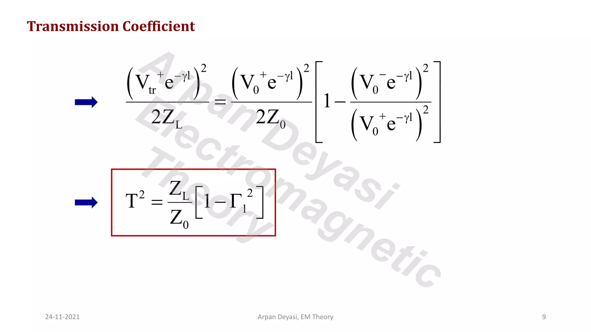
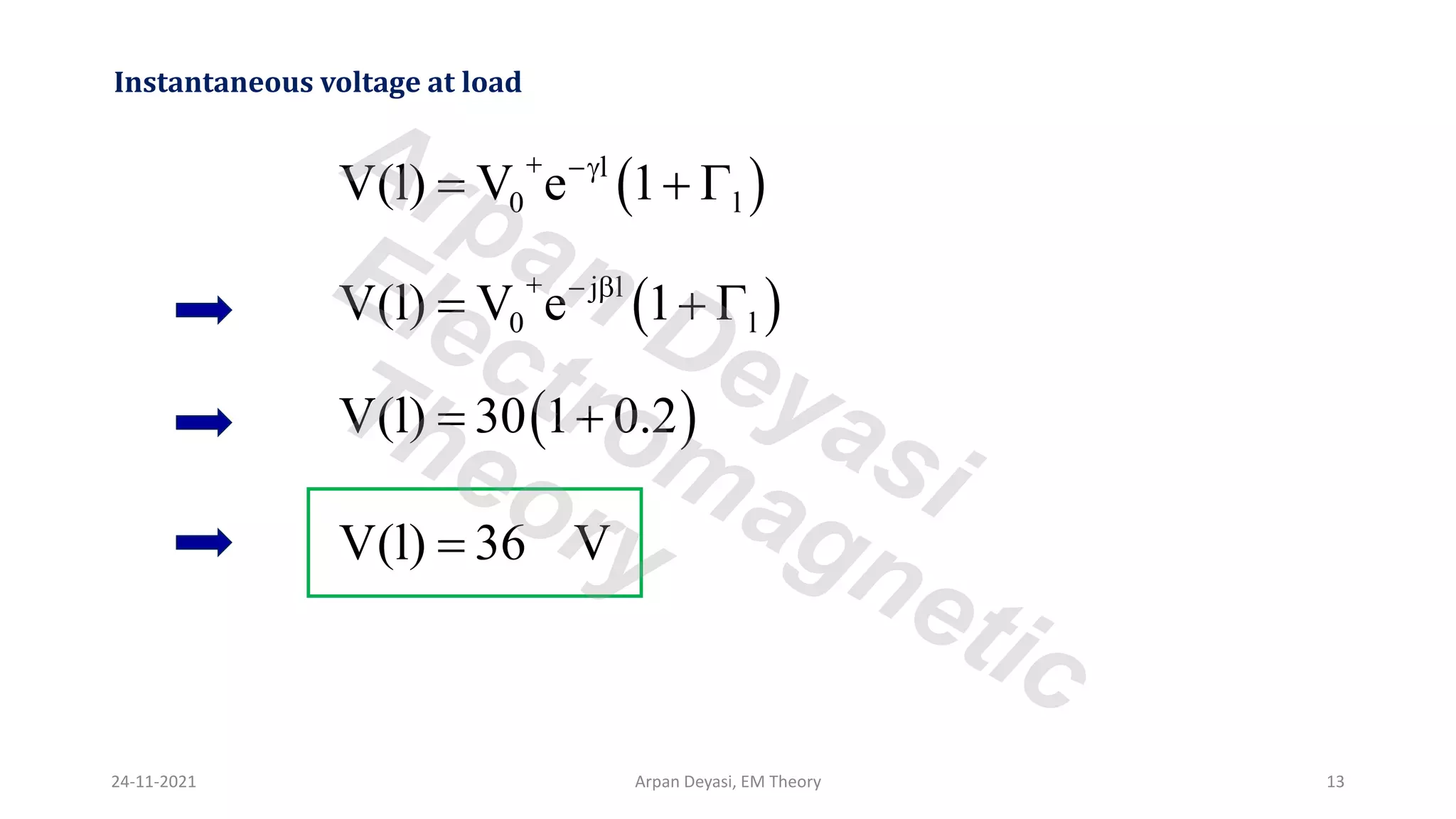
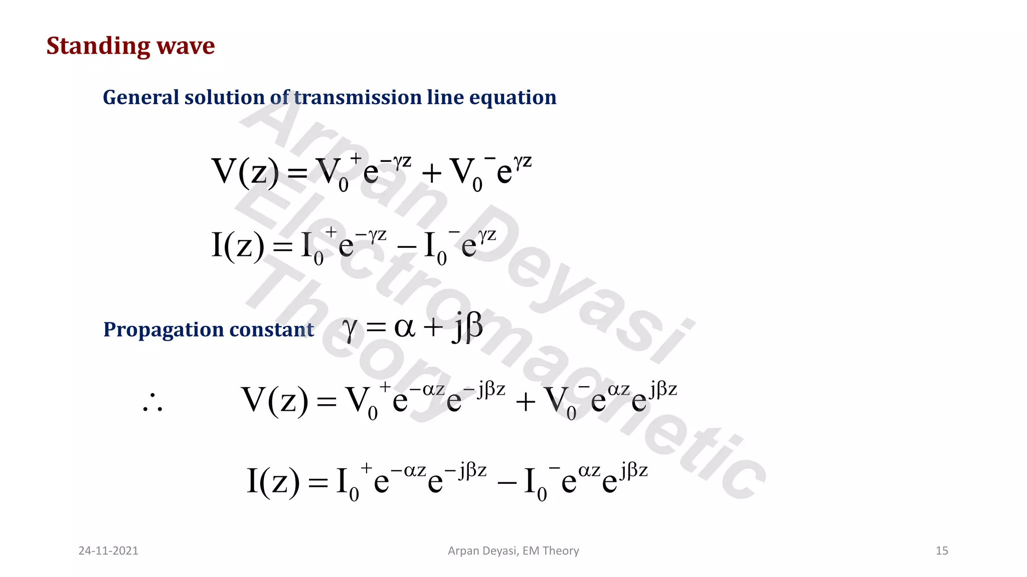
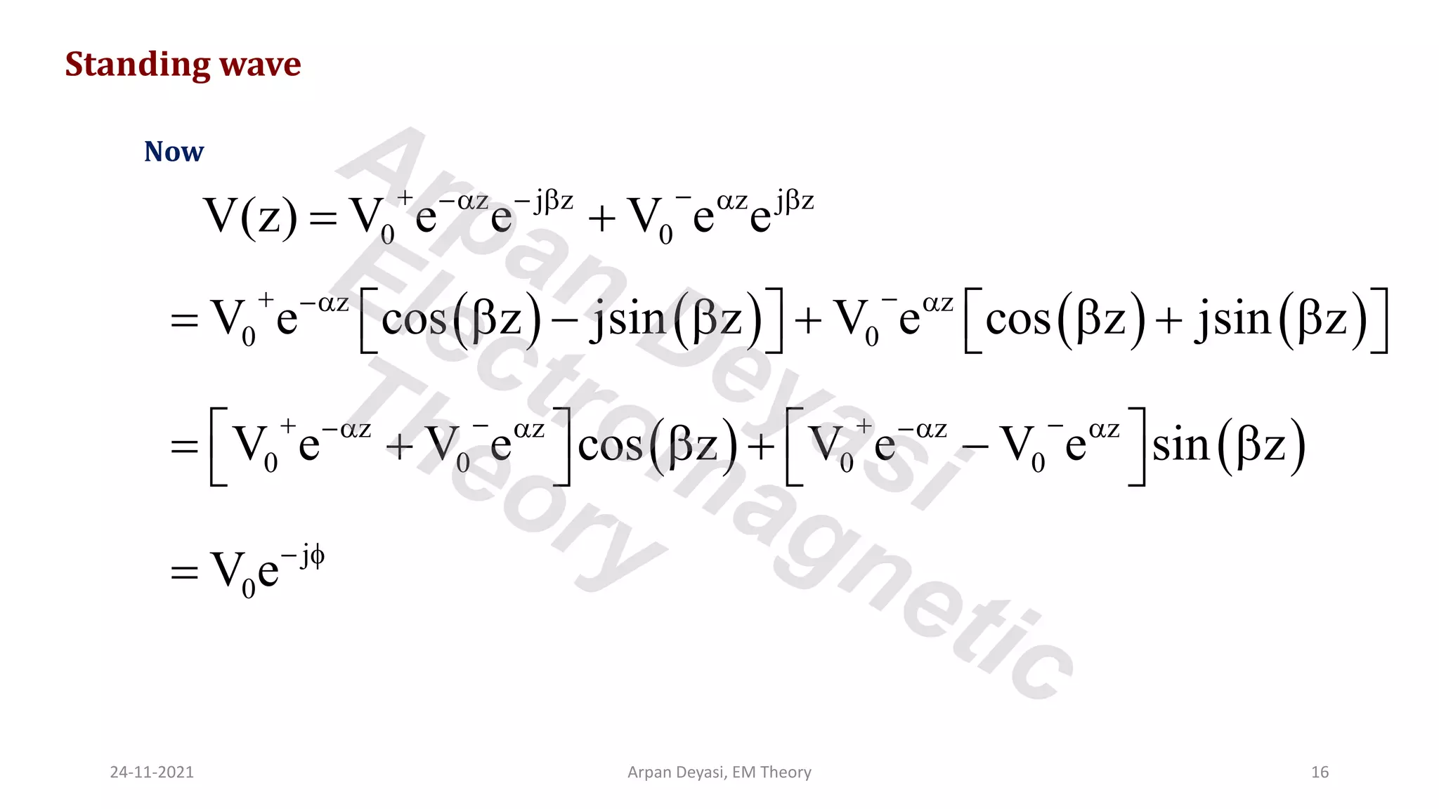
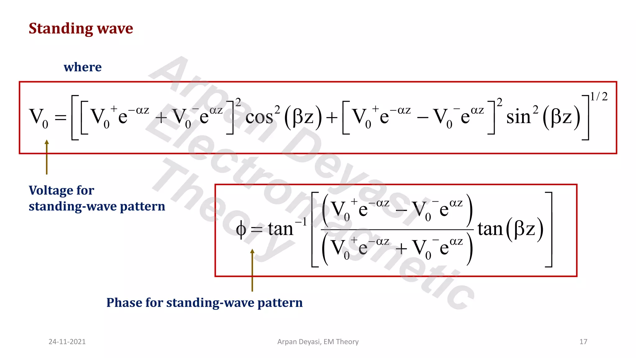
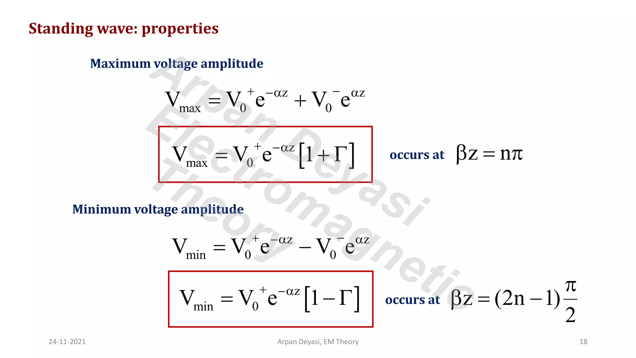
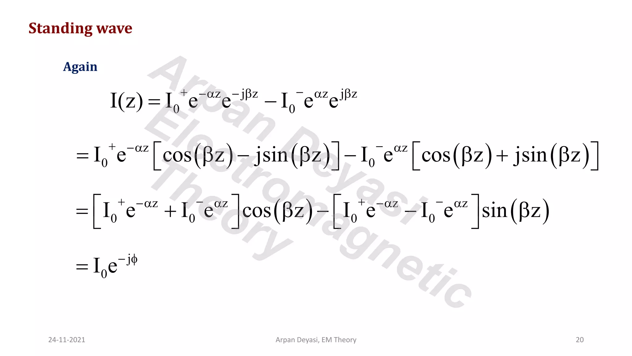
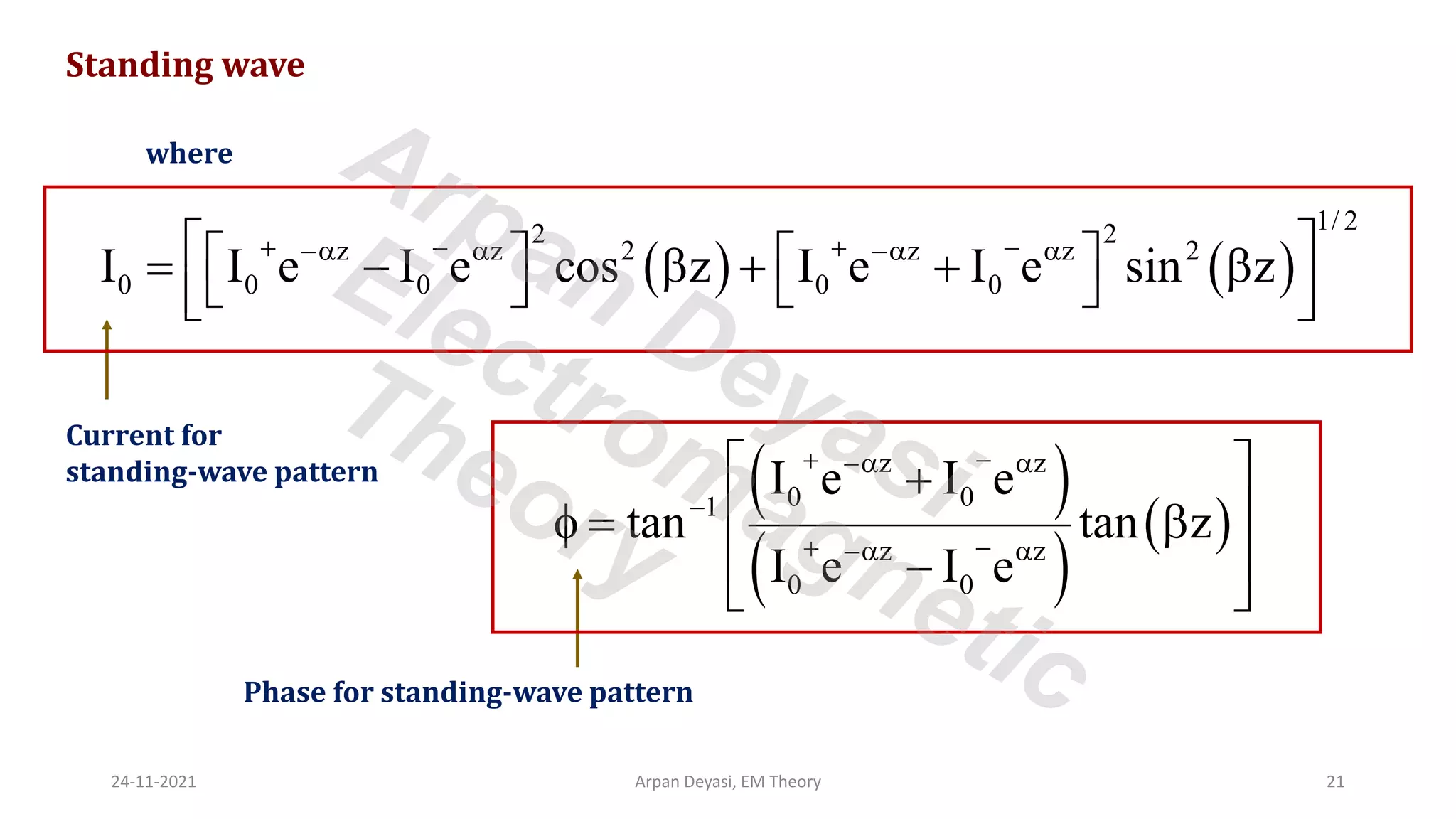
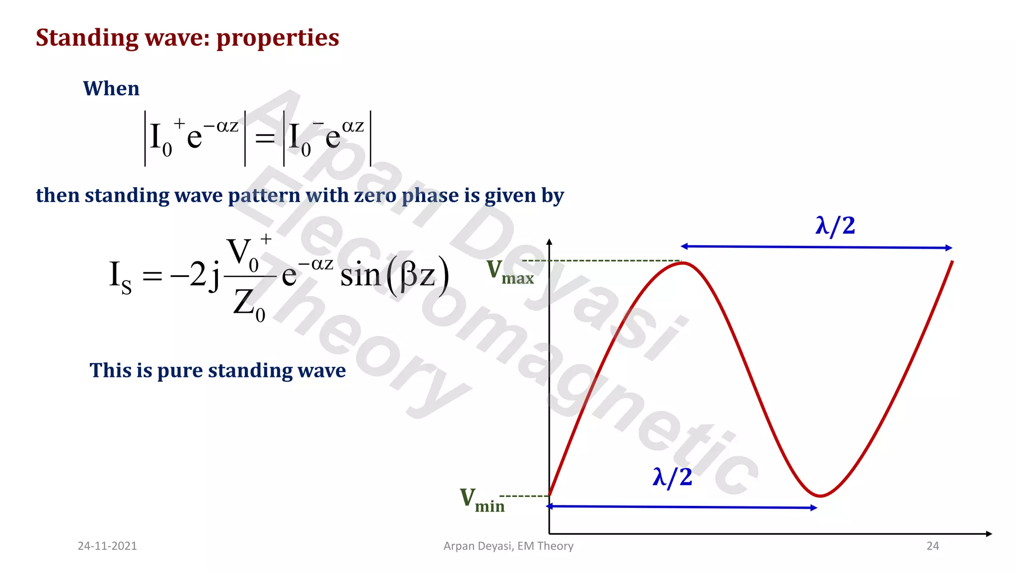
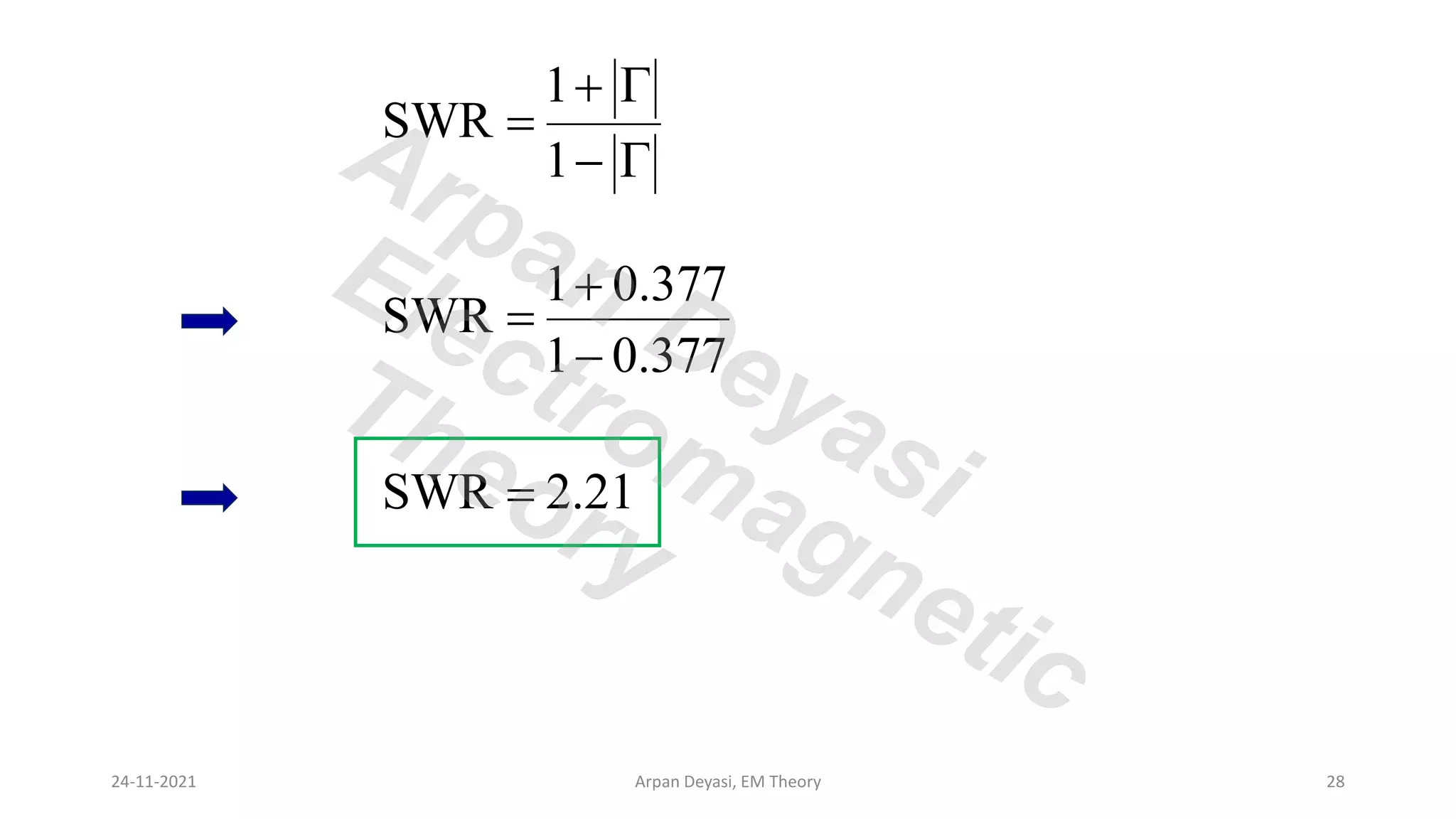
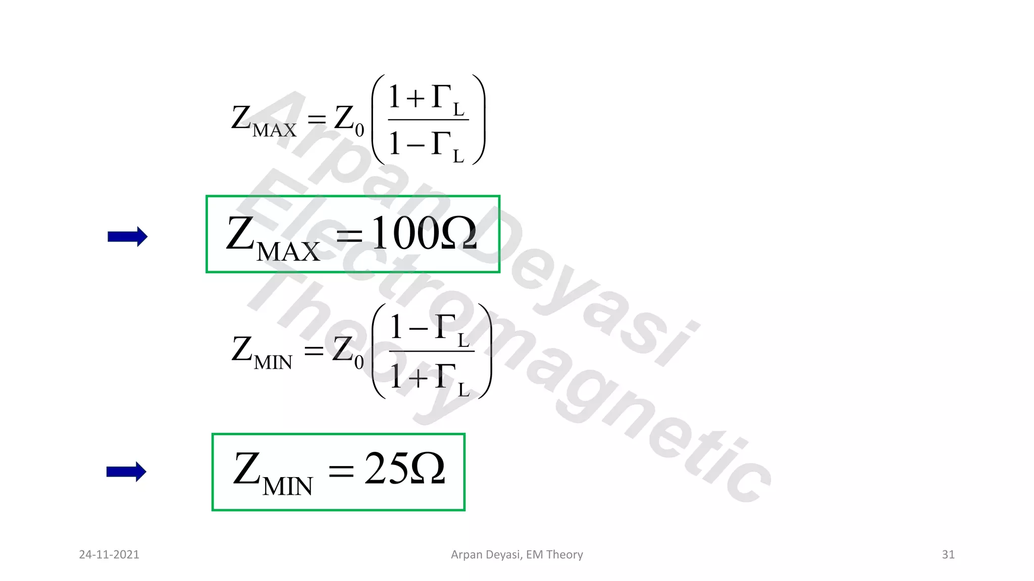
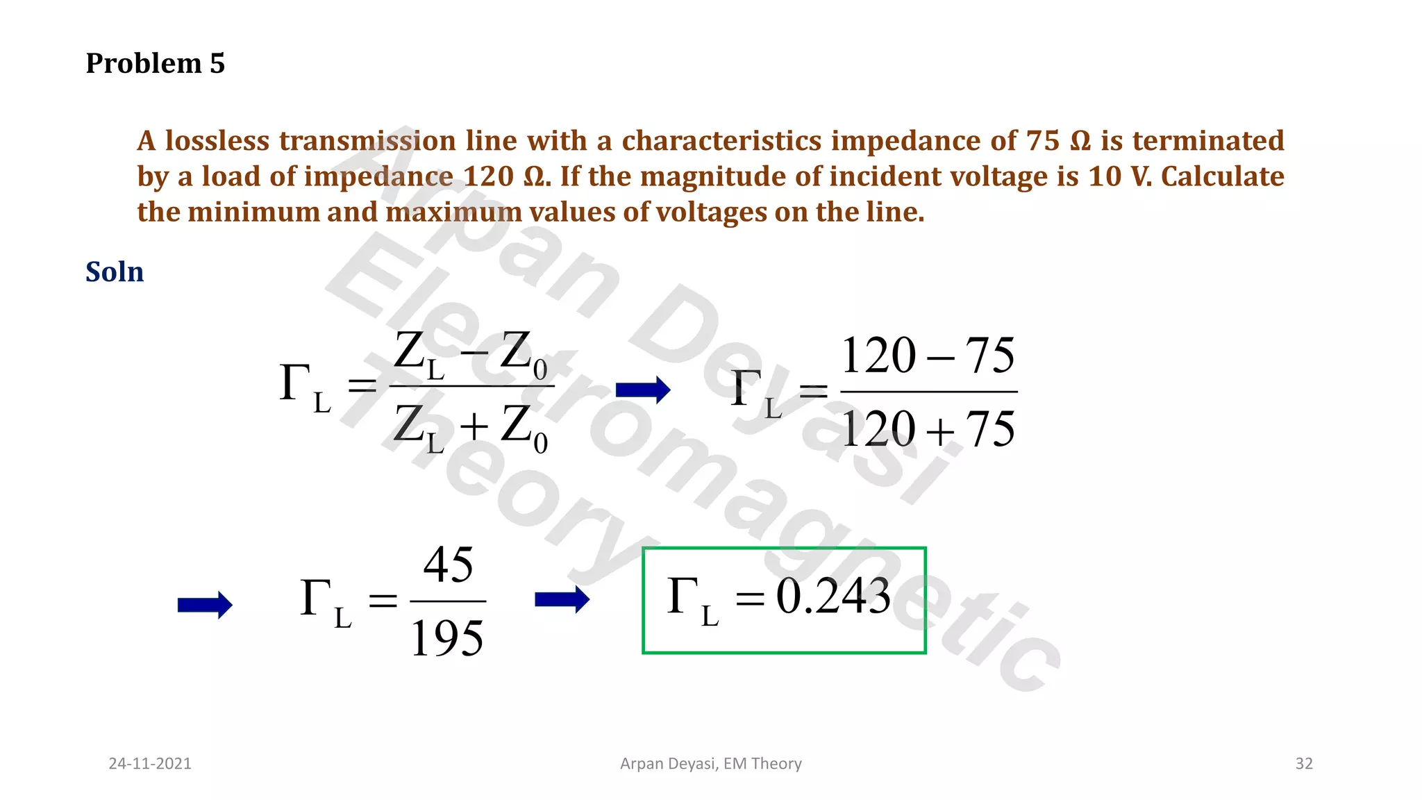
Course: Electromagnetic Theory
paper code: EI 503
Course Coordinator: Arpan Deyasi
Department of Electronics and Communication Engineering
RCC Institute of Information Technology
Kolkata, India
Topic: Transmission Line – Propagation Coefficients
24-11-2021 Arpan Deyasi, EM Theory 1
Arpan Deyasi
Electromagnetic
Theory
Reflection Coefficient
It is the ratio of reflected voltage(/current) with the incident voltage (/current)
for a given transmission line
ref ref
inc inc
V I
V I
 = = −
z
z 0 inc
inc 0
0 0
V e V
I I e
Z Z
+ −
+ −
= = =
z
z 0 ref
ref 0
0 0
V e V
I I e
Z Z
− 
− 
= = − = −
24-11-2021 Arpan Deyasi, EM Theory 2
Arpan Deyasi
Electromagnetic
Theory
Reflection Coefficient
z z
0 0
V(z) V e V e
+ −
− 
= +
Now
z z
0 0
V(z) V e V e
+ +
− −
= + 
( )
z
0
V(z) V e 1
+ −
= + 
24-11-2021 Arpan Deyasi, EM Theory 3
Arpan Deyasi
Electromagnetic
Theory
Reflection Coefficient
Similarly
z z
0 0
I(z) I e I e
+ −
− 
= −
z z
0 0
I(z) I e I e
+ +
− −
= − 
( )
z
0
I(z) I e 1
+ −
= − 
24-11-2021 Arpan Deyasi, EM Theory 4
Arpan Deyasi
Electromagnetic
Theory
Reflection Coefficient
If the transmission line has a length ‘l’
( )
l
0 l
V(l) V e 1
+ −
= + 
( )
l
0 l
I(l) I e 1
+ −
= − 
24-11-2021 Arpan Deyasi, EM Theory 5
Arpan Deyasi
Electromagnetic
Theory
Reflection Coefficient
If the transmission line is terminated by load ‘ZL’
( )
( )
l
0 l
l
0 l
V e 1
V(l)
Z(l)
I(l) I e 1
+ −
+ −
+ 
= =
− 
( )
( )
l
0
l
1
Z(l) Z
1
+ 
=
− 
L 0
l
L 0
Z Z
Z Z
−
 =
+
24-11-2021 Arpan Deyasi, EM Theory 6
Arpan Deyasi
Electromagnetic
Theory
Tranmission Coefficient
Transmission coefficient
tr tr
inc inc
V I
T
V I
= =
L 0
L 0
Z Z
T 1 1
Z Z
−
= +  = +
+
L
L 0
2Z
T
Z Z
=
+
24-11-2021 Arpan Deyasi, EM Theory 7
Arpan Deyasi
Electromagnetic
Theory
Transmission Coefficient
From power conservation principle
in ref tr
P P P
= +
tr in ref
P P P
= −
( ) ( ) ( )
2 2 2
l l l
tr 0 0
L 0 0
V e V e V e
2Z 2Z 2Z
+ + −
− − −
= −
24-11-2021 Arpan Deyasi, EM Theory 8
Arpan Deyasi
Electromagnetic
Theory
Transmission Coefficient
( ) ( ) ( )
( )
2 2 2
l l l
tr 0 0
2
l
L 0
0
V e V e V e
1
2Z 2Z V e
+ + −
− − −
+ −
 
 
= −
 
 
 
2
2 L
l
0
Z
T 1
Z
 
= − 
 
24-11-2021 Arpan Deyasi, EM Theory 9
Arpan Deyasi
Electromagnetic
Theory
Problem 1
A certain transmission line has characteristic impedance (75+j0.01) Ω and is
terminated by load impedance of (70+j50) Ω. Calculate reflection coefficient
and transmission coefficient.
Soln
L 0
l
L 0
Z Z
Z Z
−
 =
+
l
(70 j50) (75 j0.01)
(70 j50) (75 j0.01)
+ − +
 =
+ + +
l 0.08 j0.32
 = +
24-11-2021 Arpan Deyasi, EM Theory 10
Arpan Deyasi
Electromagnetic
Theory
T 1
= + 
T 1 0.08 j0.32
= + +
T 1.08 j0.32
= +
24-11-2021 Arpan Deyasi, EM Theory 11
Arpan Deyasi
Electromagnetic
Theory
Problem 2
A lossless transmission line has characteristic impedance 50 Ω and is terminated by
load impedance of 75 Ω. If the line is energized by a generator with output impedance
of 50 Ω and open circuit output voltage of 30 V [rms). Find magnitude of instantaneous
load voltage, instantaneous power delivered to the load. Consider length of the line is
2.25λ.
Soln
2
l .
4 2
  
 = =

L 0
l
L 0
Z Z 75 50
0.2
Z Z 75 50
− −
 = = =
+ +
24-11-2021 Arpan Deyasi, EM Theory 12
Arpan Deyasi
Electromagnetic
Theory
Instantaneous voltage at load
( )
l
0 l
V(l) V e 1
+ −
= + 
( )
j l
0 l
V(l) V e 1
+ − 
= + 
( )
V(l) 30 1 0.2
= +
V(l) 36 V
=
24-11-2021 Arpan Deyasi, EM Theory 13
Arpan Deyasi
Electromagnetic
Theory
Instantaneous power delivered
2
l
L
V
P(l)
Z
=
2
36
P(l)
75
=
P(l) 17.28 W
=
24-11-2021 Arpan Deyasi, EM Theory 14
Arpan Deyasi
Electromagnetic
Theory
Standing wave
General solution of transmission line equation
z z
0 0
V(z) V e V e
+ −
− 
= +
z z
0 0
I(z) I e I e
+ −
− 
= −
j
 =  + 
Propagation constant
z z
0 0
V(z) V e V e
+ −
− 
= +
z j z z j z
0 0
I(z) I e e I e e
+ −
− −   
= −
z j z z j z
0 0
V(z) V e e V e e
+ −
− −   
 = +
24-11-2021 Arpan Deyasi, EM Theory 15
Arpan Deyasi
Electromagnetic
Theory
z j z z j z
0 0
V(z) V e e V e e
+ −
− −   
= +
Standing wave
Now
( ) ( ) ( ) ( )
z z
0 0
V e cos z jsin z V e cos z jsin z
+ −
− 
=  −  +  + 
   
   
( ) ( )
z z z z
0 0 0 0
V e V e cos z V e V e sin z
+ − + −
−  − 
   
= +  + − 
   
j
0
V e− 
=
24-11-2021 Arpan Deyasi, EM Theory 16
Arpan Deyasi
Electromagnetic
Theory
Standing wave
where
( ) ( )
1/ 2
2 2
z z 2 z z 2
0 0 0 0 0
V V e V e cos z V e V e sin z
+ − + −
−  − 
 
   
= +  + − 
   
 
 
( )
( )
( )
z z
0 0
1
z z
0 0
V e V e
tan tan z
V e V e
+ −
− 
−
+ −
− 
 
−
 
 = 
 
+
 
Voltage for
standing-wave pattern
Phase for standing-wave pattern
24-11-2021 Arpan Deyasi, EM Theory 17
Arpan Deyasi
Electromagnetic
Theory
Standing wave: properties
Maximum voltage amplitude
z z
max 0 0
V V e V e
+ −
− 
= +
 
z
max 0
V V e 1
+ −
= + 
Minimum voltage amplitude
z z
min 0 0
V V e V e
+ −
− 
= −
 
z
min 0
V V e 1
+ −
= − 
occurs at z n
 = 
occurs at z (2n 1)
2

 = −
24-11-2021 Arpan Deyasi, EM Theory 18
Arpan Deyasi
Electromagnetic
Theory
Standing wave: properties
The distance between two successive minima or maxima is one-half wavelength
z n
 = 
n n
z
2
 
= =



n
z
2

=
24-11-2021 Arpan Deyasi, EM Theory 19
Arpan Deyasi
Electromagnetic
Theory
Standing wave
z j z z j z
0 0
I(z) I e e I e e
+ −
− −   
= −
Again
( ) ( ) ( ) ( )
z z
0 0
I e cos z jsin z I e cos z jsin z
+ −
− 
=  −  −  + 
   
   
( ) ( )
z z z z
0 0 0 0
I e I e cos z I e I e sin z
+ − + −
−  − 
   
= +  − − 
   
j
0
I e− 
=
24-11-2021 Arpan Deyasi, EM Theory 20
Arpan Deyasi
Electromagnetic
Theory
Standing wave
where
( ) ( )
1/ 2
2 2
z z 2 z z 2
0 0 0 0 0
I I e I e cos z I e I e sin z
+ − + −
−  − 
 
   
= −  + + 
   
 
 
( )
( )
( )
z z
0 0
1
z z
0 0
I e I e
tan tan z
I e I e
+ −
− 
−
+ −
− 
 
+
 
 = 
 
−
 
Current for
standing-wave pattern
Phase for standing-wave pattern
24-11-2021 Arpan Deyasi, EM Theory 21
Arpan Deyasi
Electromagnetic
Theory
Standing wave: properties
Maximum voltage amplitude
Minimum voltage amplitude
occurs at
occurs at
z z
max 0 0
I I e I e
+ −
− 
= −
 
z
max 0
I I e 1
+ −
= +  z n
 = 
z z
min 0 0
I I e I e
+ −
− 
= +
 
z
min 0
I I e 1
+ −
= −  z (2n 1)
2

 = −
24-11-2021 Arpan Deyasi, EM Theory 22
Arpan Deyasi
Electromagnetic
Theory
Standing wave: properties
When
z z
0 0
V e V e
+ −
− 
=
then standing wave pattern with zero phase is given by
( )
z
S 0
V 2V e cos z
+ −
= 
This is pure standing wave
Vmax
Vmin
λ/2
λ/2
24-11-2021 Arpan Deyasi, EM Theory 23
Arpan Deyasi
Electromagnetic
Theory
When
z z
0 0
I e I e
+ −
− 
=
then standing wave pattern with zero phase is given by
( )
z
0
S
0
V
I 2j e sin z
Z
+
−
= − 
This is pure standing wave
Standing wave: properties
Vmax
Vmin
λ/2
λ/2
24-11-2021 Arpan Deyasi, EM Theory 24
Arpan Deyasi
Electromagnetic
Theory
Voltage and current standing waves are 90° out of phase along any time
Standing wave: properties
Voltage nodes and current nodes are interlaced a quarter-wavelength apart
V I
λ/4
24-11-2021 Arpan Deyasi, EM Theory 25
Arpan Deyasi
Electromagnetic
Theory
Standing Wave Ratio
It is the ratio of maximum standing wave pattern (voltage/ current) to the minimum of
that value (voltage/ current)
max max
min min
V I
SWR
V I
= =
1
SWR
1
+ 
=
− 
24-11-2021 Arpan Deyasi, EM Theory 26
Arpan Deyasi
Electromagnetic
Theory
24-11-2021 Arpan Deyasi, EM Theory 27
Problem 3
A transmission line has characteristic impedance (50+j0.01) Ω and is terminated by
load impedance of (73-j42.5) Ω. Calculate SWR.
Soln
L 0
l
L 0
Z Z
Z Z
−
 =
+
l
(73 j42.5) (50 j0.01)
− − +
 =
− + +
l 0.377 42.7
 =  
Arpan Deyasi
Electromagnetic
Theory
24-11-2021 Arpan Deyasi, EM Theory 28
1
SWR
1
+ 
=
− 
1 0.377
SWR
1 0.377
+
=
−
SWR 2.21
=
Arpan Deyasi
Electromagnetic
Theory
24-11-2021 Arpan Deyasi, EM Theory 29
Problem 4
Soln
A transmission line of characteristics impedance of Z0 = 50 Ω is terminated by a load
RL = ZL = 100 Ω. Find V.S.W.R, ZMIN and ZMAX
L 0
L
L 0
Z Z
Z Z
−
 =
+
L
100 50 50
100 50 150
−
 = =
+
L 0.33
 =
Arpan Deyasi
Electromagnetic
Theory
24-11-2021 Arpan Deyasi, EM Theory 30
L
L
1
V.S.W.R
1
+ 
=
− 
1
1
3
V.S.W.R
1
1
3
+
=
−
V.S.W.R 2
=
Arpan Deyasi
Electromagnetic
Theory
24-11-2021 Arpan Deyasi, EM Theory 31
L
MAX 0
L
1
Z Z
1
 
+ 
=  
− 
 
L
MIN 0
L
1
Z Z
1
 
− 
=  
+ 
 
MAX
Z 100
= 
MIN
Z 25
= 
Arpan Deyasi
Electromagnetic
Theory
24-11-2021 Arpan Deyasi, EM Theory 32
Problem 5
Soln
A lossless transmission line with a characteristics impedance of 75 Ω is terminated
by a load of impedance 120 Ω. If the magnitude of incident voltage is 10 V. Calculate
the minimum and maximum values of voltages on the line.
L 0
L
L 0
Z Z
Z Z
−
 =
+
L
45
195
 =
L
120 75
120 75
−
 =
+
L 0.243
 =
Arpan Deyasi
Electromagnetic
Theory
24-11-2021 Arpan Deyasi, EM Theory 33
( )
Max 0 L
V V 1
= + 
( )
Min 0 L
V V 1
= − 
( )
Max
V 10 1 0.243
= +
Max
V 12.43V
=
( )
Min
V 10 1 0.243
= −
Min
V 7.57V
=
Arpan Deyasi
Electromagnetic
Theory

Reflection and Transmission coefficients in transmission line

  • 1.
    Course: Electromagnetic Theory papercode: EI 503 Course Coordinator: Arpan Deyasi Department of Electronics and Communication Engineering RCC Institute of Information Technology Kolkata, India Topic: Transmission Line – Propagation Coefficients 24-11-2021 Arpan Deyasi, EM Theory 1 Arpan Deyasi Electromagnetic Theory
  • 2.
    Reflection Coefficient It isthe ratio of reflected voltage(/current) with the incident voltage (/current) for a given transmission line ref ref inc inc V I V I  = = − z z 0 inc inc 0 0 0 V e V I I e Z Z + − + − = = = z z 0 ref ref 0 0 0 V e V I I e Z Z −  −  = = − = − 24-11-2021 Arpan Deyasi, EM Theory 2 Arpan Deyasi Electromagnetic Theory
  • 3.
    Reflection Coefficient z z 00 V(z) V e V e + − −  = + Now z z 0 0 V(z) V e V e + + − − = +  ( ) z 0 V(z) V e 1 + − = +  24-11-2021 Arpan Deyasi, EM Theory 3 Arpan Deyasi Electromagnetic Theory
  • 4.
    Reflection Coefficient Similarly z z 00 I(z) I e I e + − −  = − z z 0 0 I(z) I e I e + + − − = −  ( ) z 0 I(z) I e 1 + − = −  24-11-2021 Arpan Deyasi, EM Theory 4 Arpan Deyasi Electromagnetic Theory
  • 5.
    Reflection Coefficient If thetransmission line has a length ‘l’ ( ) l 0 l V(l) V e 1 + − = +  ( ) l 0 l I(l) I e 1 + − = −  24-11-2021 Arpan Deyasi, EM Theory 5 Arpan Deyasi Electromagnetic Theory
  • 6.
    Reflection Coefficient If thetransmission line is terminated by load ‘ZL’ ( ) ( ) l 0 l l 0 l V e 1 V(l) Z(l) I(l) I e 1 + − + − +  = = −  ( ) ( ) l 0 l 1 Z(l) Z 1 +  = −  L 0 l L 0 Z Z Z Z −  = + 24-11-2021 Arpan Deyasi, EM Theory 6 Arpan Deyasi Electromagnetic Theory
  • 7.
    Tranmission Coefficient Transmission coefficient trtr inc inc V I T V I = = L 0 L 0 Z Z T 1 1 Z Z − = +  = + + L L 0 2Z T Z Z = + 24-11-2021 Arpan Deyasi, EM Theory 7 Arpan Deyasi Electromagnetic Theory
  • 8.
    Transmission Coefficient From powerconservation principle in ref tr P P P = + tr in ref P P P = − ( ) ( ) ( ) 2 2 2 l l l tr 0 0 L 0 0 V e V e V e 2Z 2Z 2Z + + − − − − = − 24-11-2021 Arpan Deyasi, EM Theory 8 Arpan Deyasi Electromagnetic Theory
  • 9.
    Transmission Coefficient ( )( ) ( ) ( ) 2 2 2 l l l tr 0 0 2 l L 0 0 V e V e V e 1 2Z 2Z V e + + − − − − + −     = −       2 2 L l 0 Z T 1 Z   = −    24-11-2021 Arpan Deyasi, EM Theory 9 Arpan Deyasi Electromagnetic Theory
  • 10.
    Problem 1 A certaintransmission line has characteristic impedance (75+j0.01) Ω and is terminated by load impedance of (70+j50) Ω. Calculate reflection coefficient and transmission coefficient. Soln L 0 l L 0 Z Z Z Z −  = + l (70 j50) (75 j0.01) (70 j50) (75 j0.01) + − +  = + + + l 0.08 j0.32  = + 24-11-2021 Arpan Deyasi, EM Theory 10 Arpan Deyasi Electromagnetic Theory
  • 11.
    T 1 = + T 1 0.08 j0.32 = + + T 1.08 j0.32 = + 24-11-2021 Arpan Deyasi, EM Theory 11 Arpan Deyasi Electromagnetic Theory
  • 12.
    Problem 2 A losslesstransmission line has characteristic impedance 50 Ω and is terminated by load impedance of 75 Ω. If the line is energized by a generator with output impedance of 50 Ω and open circuit output voltage of 30 V [rms). Find magnitude of instantaneous load voltage, instantaneous power delivered to the load. Consider length of the line is 2.25λ. Soln 2 l . 4 2     = =  L 0 l L 0 Z Z 75 50 0.2 Z Z 75 50 − −  = = = + + 24-11-2021 Arpan Deyasi, EM Theory 12 Arpan Deyasi Electromagnetic Theory
  • 13.
    Instantaneous voltage atload ( ) l 0 l V(l) V e 1 + − = +  ( ) j l 0 l V(l) V e 1 + −  = +  ( ) V(l) 30 1 0.2 = + V(l) 36 V = 24-11-2021 Arpan Deyasi, EM Theory 13 Arpan Deyasi Electromagnetic Theory
  • 14.
    Instantaneous power delivered 2 l L V P(l) Z = 2 36 P(l) 75 = P(l)17.28 W = 24-11-2021 Arpan Deyasi, EM Theory 14 Arpan Deyasi Electromagnetic Theory
  • 15.
    Standing wave General solutionof transmission line equation z z 0 0 V(z) V e V e + − −  = + z z 0 0 I(z) I e I e + − −  = − j  =  +  Propagation constant z z 0 0 V(z) V e V e + − −  = + z j z z j z 0 0 I(z) I e e I e e + − − −    = − z j z z j z 0 0 V(z) V e e V e e + − − −     = + 24-11-2021 Arpan Deyasi, EM Theory 15 Arpan Deyasi Electromagnetic Theory
  • 16.
    z j zz j z 0 0 V(z) V e e V e e + − − −    = + Standing wave Now ( ) ( ) ( ) ( ) z z 0 0 V e cos z jsin z V e cos z jsin z + − −  =  −  +  +          ( ) ( ) z z z z 0 0 0 0 V e V e cos z V e V e sin z + − + − −  −      = +  + −      j 0 V e−  = 24-11-2021 Arpan Deyasi, EM Theory 16 Arpan Deyasi Electromagnetic Theory
  • 17.
    Standing wave where ( )( ) 1/ 2 2 2 z z 2 z z 2 0 0 0 0 0 V V e V e cos z V e V e sin z + − + − −  −        = +  + −          ( ) ( ) ( ) z z 0 0 1 z z 0 0 V e V e tan tan z V e V e + − −  − + − −    −    =    +   Voltage for standing-wave pattern Phase for standing-wave pattern 24-11-2021 Arpan Deyasi, EM Theory 17 Arpan Deyasi Electromagnetic Theory
  • 18.
    Standing wave: properties Maximumvoltage amplitude z z max 0 0 V V e V e + − −  = +   z max 0 V V e 1 + − = +  Minimum voltage amplitude z z min 0 0 V V e V e + − −  = −   z min 0 V V e 1 + − = −  occurs at z n  =  occurs at z (2n 1) 2   = − 24-11-2021 Arpan Deyasi, EM Theory 18 Arpan Deyasi Electromagnetic Theory
  • 19.
    Standing wave: properties Thedistance between two successive minima or maxima is one-half wavelength z n  =  n n z 2   = =    n z 2  = 24-11-2021 Arpan Deyasi, EM Theory 19 Arpan Deyasi Electromagnetic Theory
  • 20.
    Standing wave z jz z j z 0 0 I(z) I e e I e e + − − −    = − Again ( ) ( ) ( ) ( ) z z 0 0 I e cos z jsin z I e cos z jsin z + − −  =  −  −  +          ( ) ( ) z z z z 0 0 0 0 I e I e cos z I e I e sin z + − + − −  −      = +  − −      j 0 I e−  = 24-11-2021 Arpan Deyasi, EM Theory 20 Arpan Deyasi Electromagnetic Theory
  • 21.
    Standing wave where ( )( ) 1/ 2 2 2 z z 2 z z 2 0 0 0 0 0 I I e I e cos z I e I e sin z + − + − −  −        = −  + +          ( ) ( ) ( ) z z 0 0 1 z z 0 0 I e I e tan tan z I e I e + − −  − + − −    +    =    −   Current for standing-wave pattern Phase for standing-wave pattern 24-11-2021 Arpan Deyasi, EM Theory 21 Arpan Deyasi Electromagnetic Theory
  • 22.
    Standing wave: properties Maximumvoltage amplitude Minimum voltage amplitude occurs at occurs at z z max 0 0 I I e I e + − −  = −   z max 0 I I e 1 + − = +  z n  =  z z min 0 0 I I e I e + − −  = +   z min 0 I I e 1 + − = −  z (2n 1) 2   = − 24-11-2021 Arpan Deyasi, EM Theory 22 Arpan Deyasi Electromagnetic Theory
  • 23.
    Standing wave: properties When zz 0 0 V e V e + − −  = then standing wave pattern with zero phase is given by ( ) z S 0 V 2V e cos z + − =  This is pure standing wave Vmax Vmin λ/2 λ/2 24-11-2021 Arpan Deyasi, EM Theory 23 Arpan Deyasi Electromagnetic Theory
  • 24.
    When z z 0 0 Ie I e + − −  = then standing wave pattern with zero phase is given by ( ) z 0 S 0 V I 2j e sin z Z + − = −  This is pure standing wave Standing wave: properties Vmax Vmin λ/2 λ/2 24-11-2021 Arpan Deyasi, EM Theory 24 Arpan Deyasi Electromagnetic Theory
  • 25.
    Voltage and currentstanding waves are 90° out of phase along any time Standing wave: properties Voltage nodes and current nodes are interlaced a quarter-wavelength apart V I λ/4 24-11-2021 Arpan Deyasi, EM Theory 25 Arpan Deyasi Electromagnetic Theory
  • 26.
    Standing Wave Ratio Itis the ratio of maximum standing wave pattern (voltage/ current) to the minimum of that value (voltage/ current) max max min min V I SWR V I = = 1 SWR 1 +  = −  24-11-2021 Arpan Deyasi, EM Theory 26 Arpan Deyasi Electromagnetic Theory
  • 27.
    24-11-2021 Arpan Deyasi,EM Theory 27 Problem 3 A transmission line has characteristic impedance (50+j0.01) Ω and is terminated by load impedance of (73-j42.5) Ω. Calculate SWR. Soln L 0 l L 0 Z Z Z Z −  = + l (73 j42.5) (50 j0.01) (73 j42.5) (50 j0.01) − − +  = − + + l 0.377 42.7  =   Arpan Deyasi Electromagnetic Theory
  • 28.
    24-11-2021 Arpan Deyasi,EM Theory 28 1 SWR 1 +  = −  1 0.377 SWR 1 0.377 + = − SWR 2.21 = Arpan Deyasi Electromagnetic Theory
  • 29.
    24-11-2021 Arpan Deyasi,EM Theory 29 Problem 4 Soln A transmission line of characteristics impedance of Z0 = 50 Ω is terminated by a load RL = ZL = 100 Ω. Find V.S.W.R, ZMIN and ZMAX L 0 L L 0 Z Z Z Z −  = + L 100 50 50 100 50 150 −  = = + L 0.33  = Arpan Deyasi Electromagnetic Theory
  • 30.
    24-11-2021 Arpan Deyasi,EM Theory 30 L L 1 V.S.W.R 1 +  = −  1 1 3 V.S.W.R 1 1 3 + = − V.S.W.R 2 = Arpan Deyasi Electromagnetic Theory
  • 31.
    24-11-2021 Arpan Deyasi,EM Theory 31 L MAX 0 L 1 Z Z 1   +  =   −    L MIN 0 L 1 Z Z 1   −  =   +    MAX Z 100 =  MIN Z 25 =  Arpan Deyasi Electromagnetic Theory
  • 32.
    24-11-2021 Arpan Deyasi,EM Theory 32 Problem 5 Soln A lossless transmission line with a characteristics impedance of 75 Ω is terminated by a load of impedance 120 Ω. If the magnitude of incident voltage is 10 V. Calculate the minimum and maximum values of voltages on the line. L 0 L L 0 Z Z Z Z −  = + L 45 195  = L 120 75 120 75 −  = + L 0.243  = Arpan Deyasi Electromagnetic Theory
  • 33.
    24-11-2021 Arpan Deyasi,EM Theory 33 ( ) Max 0 L V V 1 = +  ( ) Min 0 L V V 1 = −  ( ) Max V 10 1 0.243 = + Max V 12.43V = ( ) Min V 10 1 0.243 = − Min V 7.57V = Arpan Deyasi Electromagnetic Theory