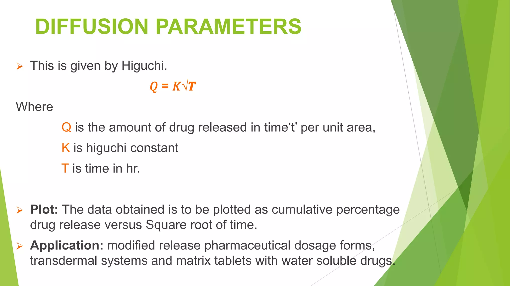
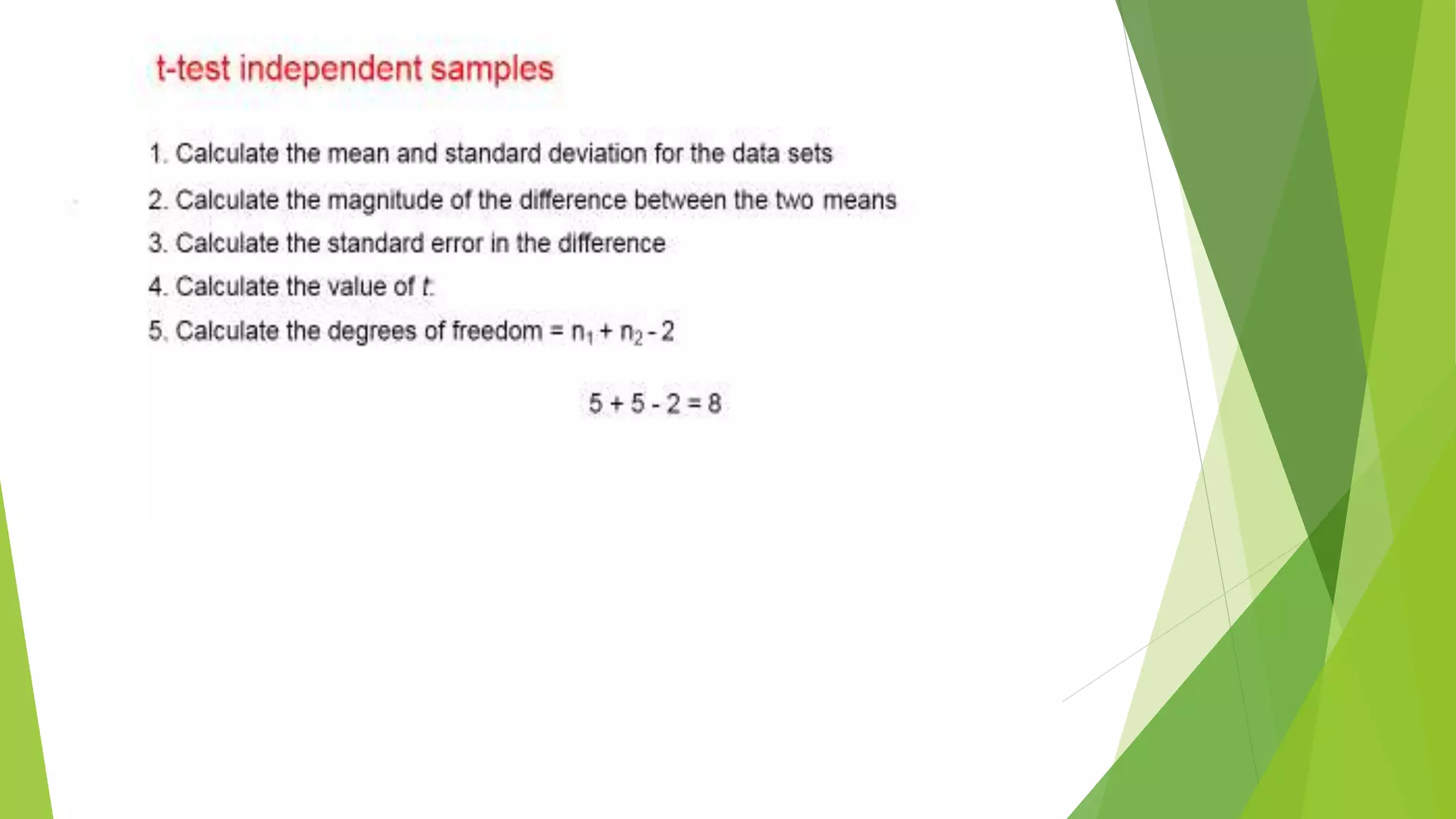
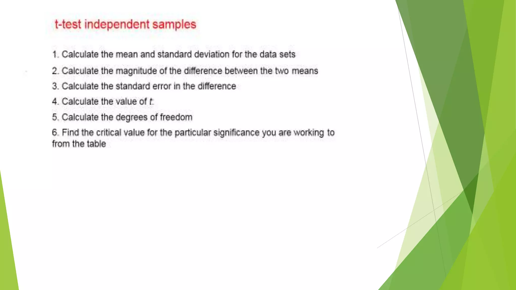
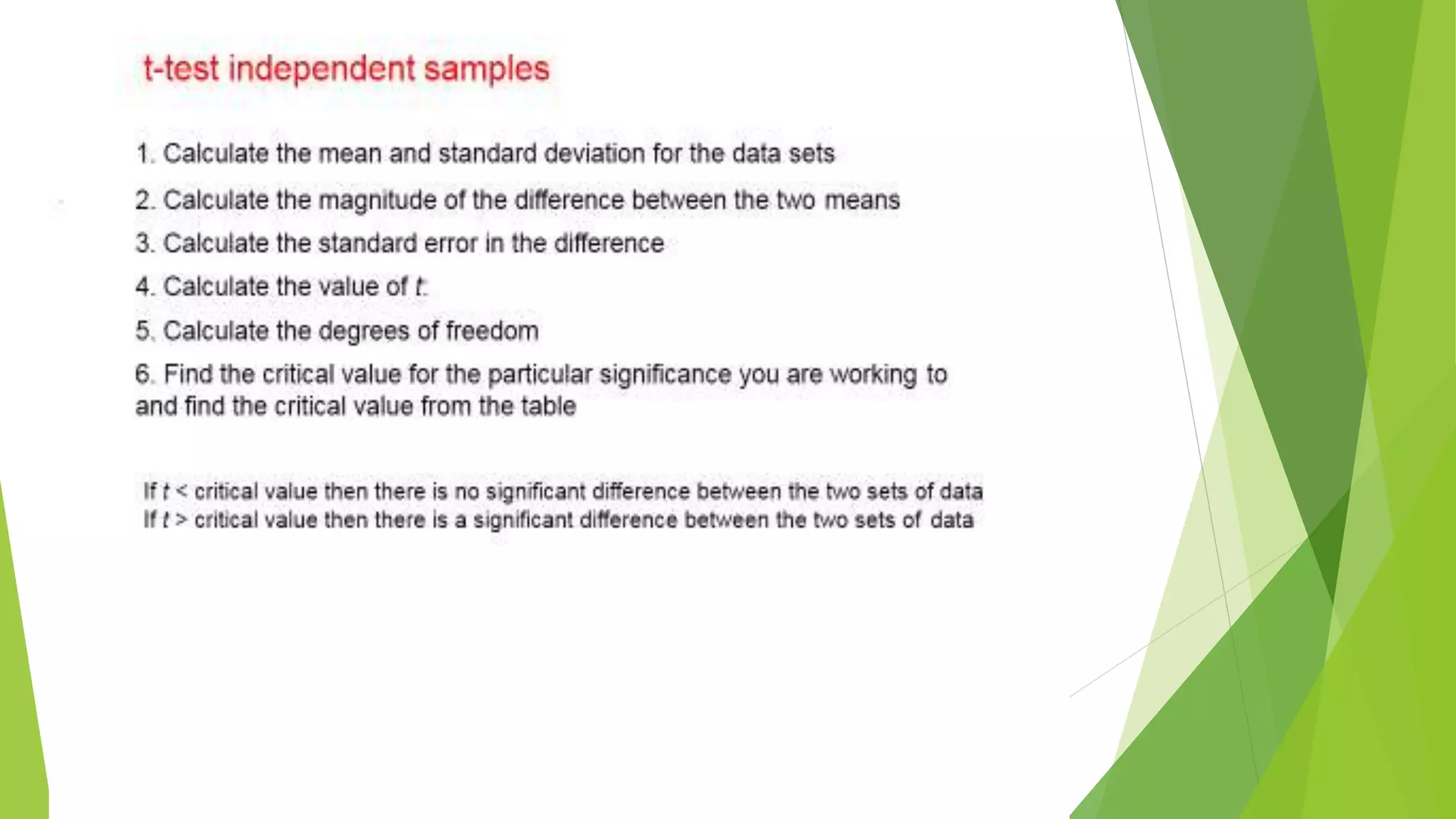
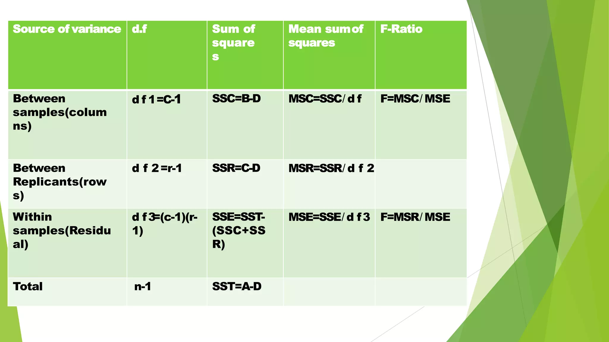
The document focuses on consolidation parameters in pharmaceutical sciences, detailing processes such as cold welding and fusion bonding, alongside various mechanisms impacting mechanical strength. It also explores diffusion and dissolution parameters critical for drug release, including effects of agitation, viscosity, and pH. Additionally, it covers pharmacokinetics, statistical methods including chi-square tests, student’s t-test, and ANOVA for analyzing data relevant to drug formulation and efficacy.

1. STUDY OF
CONSOLIDATION
PARAMETERS
By
P. viji
M.Pharm I Year
(pharmaceutics)

2. CONSOLIDATION
 An increase in the mechanical strength of the
material resulting from particle or particle
interaction. ( Increasing in mechanical strength of
the mass)

3. CONSOLIDATION PROCESS
Cold welding:
 when the surfaces of two particles approach each other
closely enough, their free surface energies results in strong
attractive force, a process known as cold welding.
Fusion bonding:
 Multiple point contacts of the particle upon application of
load produces heat which causes fusion / melting. Upon
removal of load it gets solidified and increase the mechanical
strength of mass.

5. CONSOLIDATION MECHANISMS
Mechanical theory:
 As the particles undergo deformation, the particle boundaries
that the edges of the particle intermesh, forming a mechanical
bond.
Intermolecular forces theory:
 Under pressure the molecules at the point of true contact
between new, clean surface of the granules are close enough so
that van der Waals forces interact to consolidate the particle.

6. Liquid-surface film theory:
 Thin liquid films form which bond the particles together at the
particle surface. The energy of compression produces melting of
solution at the particle interface followed by subsequent
solidification or crystallization thus resulting in the formation of
bonded surfaces

7. FACTORS AFFECTING CONSOLIDATION:
 The chemical nature of the material
 The extent of the available surface
 The presence of surface contaminants
 The inter surface distance

8. DIFFUSION PARAMETERS

9. DIFFUSION PARAMETERS
 This is given by Higuchi.
𝑄 = 𝐾√𝑻
Where
Q is the amount of drug released in time‘t’ per unit area,
K is higuchi constant
T is time in hr.
 Plot: The data obtained is to be plotted as cumulative percentage
drug release versus Square root of time.
 Application: modified release pharmaceutical dosage forms,
transdermal systems and matrix tablets with water soluble drugs.

10. DISSOLUTION PARAMETERS

11. DISSOLUTION PARAMETERS
 Dissolution is a process in which a solid substance solubilizes in a given
solvent i.e. mass transfer from the solid surface to the liquid phase.
Dissolution parameters:
Effect of agitation
Effect of dissolution fluid
Influence of pH of dissolution fluid

12. Effect of viscosity of the dissolution medium
Effect of the presence of unreactive and reactive additives in the dissolution
medium.
Volume of dissolution medium and sink conditions
Deaeration of the dissolution medium
Effect of temperature of the dissolution medium

13. EFFECT OF AGITATION
 The relationship between the intensity of agitation and the
rate of dissolution varies considerably according to the type
of agitation used, the shape and design of the stirrer and
the physicochemical properties of the solid.
 For the basket method, 100 rpm usually is utilized, while for
the paddle procedure, a 50 – 75 rpm is recommended.

14. EFFECT OF DISSOLUTION FLUID
 Selection of proper medium for dissolution testing depends
largely on the physicochemical properties of the drug.

15. INFLUENCE OF PH OF DISSOLUTION
FLUID
 simulated gastric fluid as the test medium for tablets containing
ingredients which reacted more readily in acid solution than in
water (e.g., calcium carbonate).

16. EFFECT OF VISCOSITY OF THE
DISSOLUTION MEDIUM
 If the interaction at the interfaces, occurs much faster than the rate
of transport, such as in the case of diffusion controlled dissolution
processes, it would be expected that the dissolution rate decreases
with an increase in viscosity.
 The rate of dissolution of zinc in HCl solution containing
sucrose was inversely proportional to the viscosity of solution.

17. EFFECT OF THE PRESENCE OF UNREACTIVE AND
REACTIVE ADDITIVES IN THE DISSOLUTION
MEDIUM.
 When neutral ionic compounds, such as sodium chloride and
sodium sulfate, or non ionic organic compounds, such as
dextrose, were added to the dissolution medium,the dissolution
of benzoic acid was dependent linearly upon its solubility in the
particular solvent.
 When certain buffers or bases were added to the aqueous
solvent , an increase in the dissolution rate was observed.

18. VOLUME OF DISSOLUTION MEDIUM
AND SINK CONDITIONS
 The proper volume of the dissolution medium depends mainly
on the solubility of the drug in the selected fluid.
 If the drug is poorly soluble in water, a relatively large amount
of fluid should be used if complete dissolution is to be
expected.

19. DEAERATION OF THE DISSOLUTION
MEDIUM
 Presence of dissolved air or other gases in the dissolution
medium may influence the dissolution rate of certain
formulations and lead to variable and unreliable results.
 Example, the dissolved air in distilled water could significantly
lower its pH and consequently affect the dissolution rate of
drugs that are sensitive to pH changes, e.g., weak acids.

20. EFFECT OF TEMPERATURE OF THE
DISSOLUTION MEDIUM
 Drug solubility is temperature dependent, therefore careful
temperature control during the dissolution process is extremely
important.
 Generally a temperature of 37°±0.5 is maintained during
dissolution determination of oral dosage forms and suppositories.
 For topical preparations as low as 30° and 25°have been used.

21. PHARMACOKINETIC
PARAMETERS

22. PHARMACOKINETIC PARAMETERS
 Pharmacokinetics is defined as the kinetics of drug absorption,
distribution, metabolism, and excretion and their relationship
with pharmacologic, therapeutic or toxicologic response in
mans and animals.

23. PLASMA DRUG CONCENTRATION-TIME
PROFILE

24. Three important pharmacokinetic parameters:
 Peak plasma concentration (Cmax)
 Time of peak concentration (tmax)
 Area under the curve (AUC)

25. PEAK PLASMA CONCENTRATION (Cmax)
 The point of maximum concentration of a drug in plasma is called
as peak and the concentration of drug at peak is known as peak
plasma concentration.
 It is also called as peak height concentration and maximum drug
concentration.
 Cmax is expressed in mcg/ml.

26. TIME OF PEAK CONCENTRATION (tmax)
 The time for drug to reach peak concentration in plasma ( after
extravascular administration) is called the time of peak
concentration.
 It is expressed in hours.

27. AREA UNDER THE CURVE (AUC)
 It represents the total integrated area under the plasma level-
time profile and expresses the total amount of drug that comes
into the systemic circulation after its administration.
 AUC is expressed in mcg/ml X HRS.
 It is important for the dugs that are administered repetitively for
the treatment of chronic conditions like asthma or epilepsy.

28. SIMILARITY FACTORS f1 AND f2

29. SIMILARITY FACTORS f1 AND f2
DIFFERENCE FACTOR (f1)
 The difference factor (f1) as defined by FDA calculates the %
difference between 2 curves at each time point and is a
measurement of the relative error between 2 curves.
where,
n = number of time points
Rt = % dissolved at time t of reference product (prechange)
Tt = % dissolved at time t of test product (post change)

30. SIMILARITY FACTOR (F2)
 The similarity factor (f2) as defined is a measurement of the
similarity in the percentage (%) dissolution between the
two curves

31. LIMITS FOR SIMILARITY AND DIFFERENCE
FACTORS
Inference
Dissolutions profile
are similar
Similarity or
equivalence of two
profiles
≥50≤15
0 100
Differencefactor Similarityfactor

32. Data structure and steps to follow:
 This model-independent method is most suitable for the
dissolution profile comparison when three to four or more
dissolution time points are available.
 Determine the dissolution profile of two products (12 units each)
of the test (post-change) and reference (pre-change) products.

33. Some recommendations:
 The dissolution measurements of the test and reference
batches should be made under exactly the same conditions.
 The dissolution time points for both the profiles should be the
same (e.g. 15, 30, 45, 60 minutes).

34. Advantages
 They are easy to compute.
 They provide a single number to describe the comparison of
dissolution profile data.
Disadvantages
 The basis of the criteria for deciding the difference or
similarity between dissolution profile is unclear.

35. HECKEL PLOTS

36. HECKEL EQUATION
 The heckel analysis is a most popular method of deforming
reduction under compression pressure .
 Powder packing with increasing compression load is normally
attributed to particles rearrangement , elastic & plastic
deformation & particle fragmentation.

37.  It is analogous to first order reaction ,
Log 1/E= Ky . P + Kr
Where
Ky =material dependent constant inversely proportional to
its yield strength ‘s’
Kr=initial repacking stage hence E0

38.  The applied compressional force F & the movement of the
punches during compression cycle & applied pressure P , porosity
E.
For a cylindrical tablets
p=4F/л. D2
Where…
D is the tablet diameter similarly E can be calculated by
E=100.(1-4w/ρt .л.D2.H)
Where…
w is the weight of the tableting mass ,
ρt is its true density ,
H is the thickness of the tablets.

39. HECKEL PLOTS
 Heckel plot is density v/s applied pressure
 Follows first order kinetics
 Materials that are comparatively soft & that readily undergo plastic
deformation retain different degree of porosity , depending upon
the initial packing in the die.

40.  This in turn is influenced by the size distribution , shape etc of
the original particles.
 Ex: sodium chloride (shown by type a in graph)
 Harder material with higher yield pressure values usually
undergo compression by fragmentation first , to provide a
denser packing.
 Ex: Lactose, sucrose ( shown in type b in graph).

41.  Type-a plots exhibits higher slop (Ky) then type-b. because
type-a materials have lower yield stress.
 Type-b plots exhibits lower slop because brittle , hard
materials are more difficult to compress.

42. APPLICATION OF HECKEL EQUATION
 The crushing strength of tablets can be correlated with the values of
k of the Heckel plot .
 Larger k values usually indicate harder tablets.
 Such information can be used as a means of binder
selection when designing tablet formulations.
 Heckel plots can be influenced by the overall time of compression,
the degree of lubrication and even the size of the die, so that the
effects of these variables are also important and should be taken
into consideration

43. HIGUCHI MODEL

44. HIGUCHI MODEL
 The first example of a mathematical model aimed to describe drug
release from a matrix system was proposed by Huguchi in 1961.
 This model is based on the hypothesis that
(i) drug diffusion takes place only in one dimension
(ii) drug particles are much smaller than system
thickness
(iii) drug diffusivity is constant
(iv) perfect sink conditions are always attained in the
release environment.

45.  Accordingly, model expression is given by the equation:
ft = Q = A √D(2C ñ Cs) Cs t
 where
Q is the amount of drug released in time
t per unit area A,
C is the drug initial concentration,
Cs is the drug solubility in the matrix media and
D is the diffusivity of the drug molecules (diffusion coefficient)
in the matrix substance.

46.  In a general way it is possible to simplify the Higuchi model as
(generally known as the simplified Higuchi model):
f t = Q = KH x t1/2
where,
KH is the Higuchi dissolution constant.
 The data obtained were plotted as cumulative percentage drug
release versus square root of time .
 Application: This relationship can be used to describe the drug
dissolution from several types of modified release
pharmaceutical dosage forms, as in the case of some
transdermal systems and matrix tablets with water soluble
drugs.

47. KORSMEYER-PEPPAS MODEL

48. KORSMEYER-PEPPAS MODEL
 Korsmeyer et al. (1983) derived a simple relationship which
described drug release from a polymeric system equation .
 To find out the mechanism of drug release, first 60% drug release
data were fitted in Korsmeyer-Peppas model

49. Mt / M∞ = Ktn
where
Mt / M∞ is a fraction of drug released at time t,
k is the release rate constant and
n is the release exponent.
 The n value is used to characterize different release for
cylindrical shaped matrices.

50.  To find out the exponent of n the portion of the release curve,
where
Mt / M∞ < 0.6
should only be used.
 To study the release kinetics, data obtained from in vitro
drug release studies were plotted as log cumulative
percentage drug release versus log time.

52. CHI-SQUARE TEST

53. CHI-SQUARE TEST
 Karl Pearson introduced a test to distinguish whether an
observed set of frequencies differs from a specified
frequency distribution
 The chi-square test uses frequency data to generate a
statistic

54. Parametric
Test for
comparing
variance
Non-Parametric
Testing
Independence
Test for
Goodness of Fit
Chi-Square Test

55. Test for comparing variance
Chi- Square Test as a Parametric Test

56. Chi- Square Test as a Non-Parametric
Test
 Test of Goodness of Fit.
 Test of Independence.

58. 2.AS A TEST OF GOODNESS OF
FIT
 It enables us to see how well does the assumed theoretical
distribution(such as Binomial distribution, Poisson
distribution or Normal distribution) fit to the observed data.
When the calculated value of χ2 is less than the table
value at certain level of significance, the fit is considered
to be good one and if the calculated value is greater than
the table value, the fit is not considered to be good.

60. 3.AS A TEST OF INDEPENDENCE
 χ2 test enables us to explain whether or not two attributes
are associated. Testing independence determines whether
two or more observations across two populations are
dependent on each other (that is, whether one variable
helps to estimate the other. If the calculated value is less
than the table value at certain level of significance for a
given degree of freedom, we conclude that null hypotheses
stands which means that two attributes are independent or
not associated. If calculated value is greater than the table
value, we reject the null hypotheses.

61. Steps involved
1)Determine The Hypothesis:
 Ho : The two variables are independent
 Ha : The two variables are associated
2) Calculate Expected frequency

63. 3)

65. 4)determine degrees of freedom
df = (R-1)(C-1) =
(2-1)(3-1)= 2

66. 5)Compare computed test statistic
against a tabled/critical value
 If calculated 2 is greater than 2 table value, reject Ho

67. Student’s t-test

68. Student’s t-test
 The test is used to compare samples from two different
batches.
 It is usually used with small (<30) samples that are
normally distributed.

69. There are two types of t-test:
 Matched pairs
 independent pairs

121. ANALYSIS OF VARIANCE
(ANOVA)

122. ANALYSIS OF VARIANCE
(ANOVA)
 The analysis of variance(ANOVA) is developed by
R.A.Fisher in 1920.
 The technique of variance analysis developed by fisher is
very useful in such cases and with its help it is possible to
study the significance of the difference of mean values of a
large no.ofsamples at the same time.

123. CLASSIFICATION OF ANOVA
 The Analysis of variance is classified into two ways:
 One-way classification
 Two-way classification
In a one-way classification we take into account the
effect of only one variable.
If there is a two way classification the effect of two
variables can be studied.

124. One Way ANOVA
Steps
1. State null & alternative hypothesis
2.State Alpha
3.Calculate degrees of Freedom
4.State decision rule
5. Calculate test statistic
6.Calculate F statistic

126. 1)Null hypothesis
 No significant difference in the means of 3 samples
2)State Alpha i.e 0.05
3)Calculate degrees of Freedom
k-1 & n-k= 2 & 12
4)State decision rule
 Table value of F at 5% level of significance for d.f 2 & 12
is
3.88
 The calculated value of F > 3.88 ,H0 will be rejected

127. 5) Calculate test statistic

129. Sum of squares between samples (SSC)
Sum of squares between samples (SSC) =
n1 (M1 – Grand avg)2+n2 (M2– Grand avg)2+n3(M3– Grandavg)2
5 ( 10- 10)2 + 5( 8- 10)2 + 5 ( 12- 10)2 =40

130. Sum of squares WITH IN samples

131. Calculation of ratio F

132. Two Way ANOVA
Example
 we have test score of boys & girls in age group of 10 yr,11yr &
12 yr. If we want to study the effect of gender & age on score.
 Two independent factors- Gender, Age Dependent factor -
Test score

133. Source of variance d.f Sum of
square
s
Mean sumof
squares
F-Ratio
Between
samples(colum
ns)
d f 1=C-1 SSC=B-D MSC=SSC̸ d f F=MSC̸ MSE
Between
Replicants(row
s)
d f 2=r-1 SSR=C-D MSR=SSR̸ d f 2
Within
samples(Residu
al)
d f3=(c-1)(r-
1)
SSE=SST-
(SSC+SS
R)
MSE=SSE̸ d f3 F=MSR̸ MSE
Total n-1 SST=A-D

134. APPLICATIONS OF ANOVA
 Similar to t-test
 More versatile than t-test
 ANOVA is the synthesis of several ideas & it is used for
multiple purposes.
 The statistical Analysis depends on the design and
discussion of ANOVA therefore includes common statistical
designs used in pharmaceutical research

135.  In the bioequivalence studies the similarities between the
samples will be analyzed with ANOVA only.
 Pharmacokinetic data also will be evaluated using ANOVA.
 Pharmacodynamics (what drugs does to the body) data
also will be analyzed with ANOVA only.