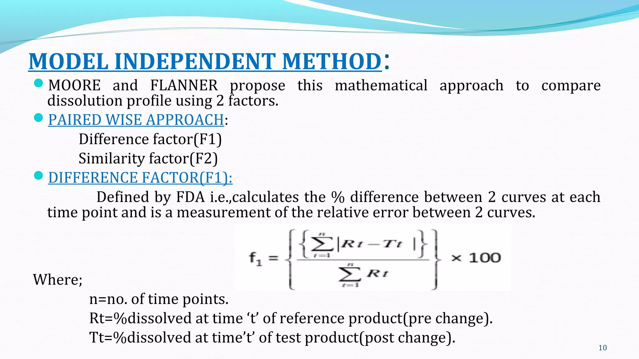
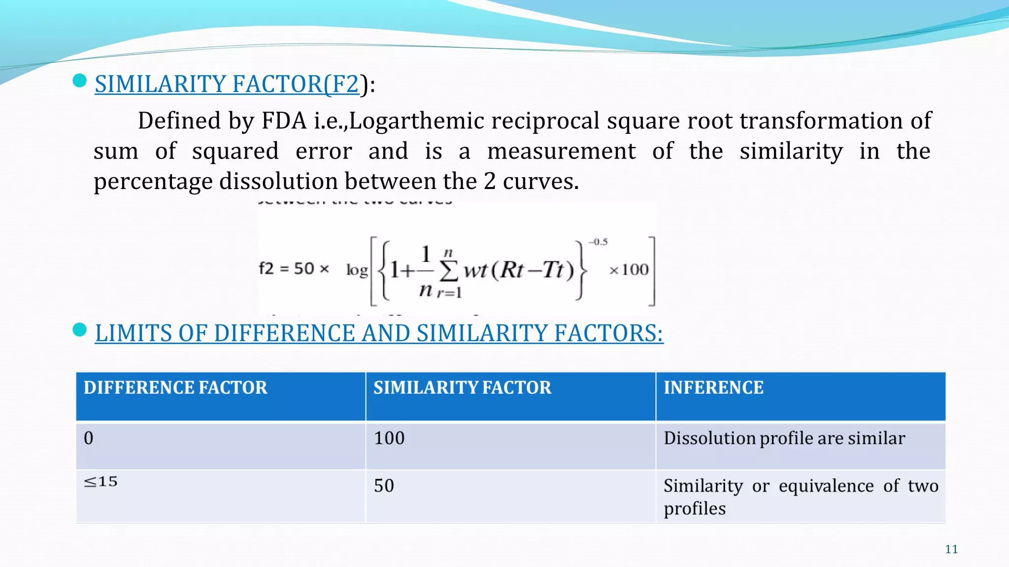
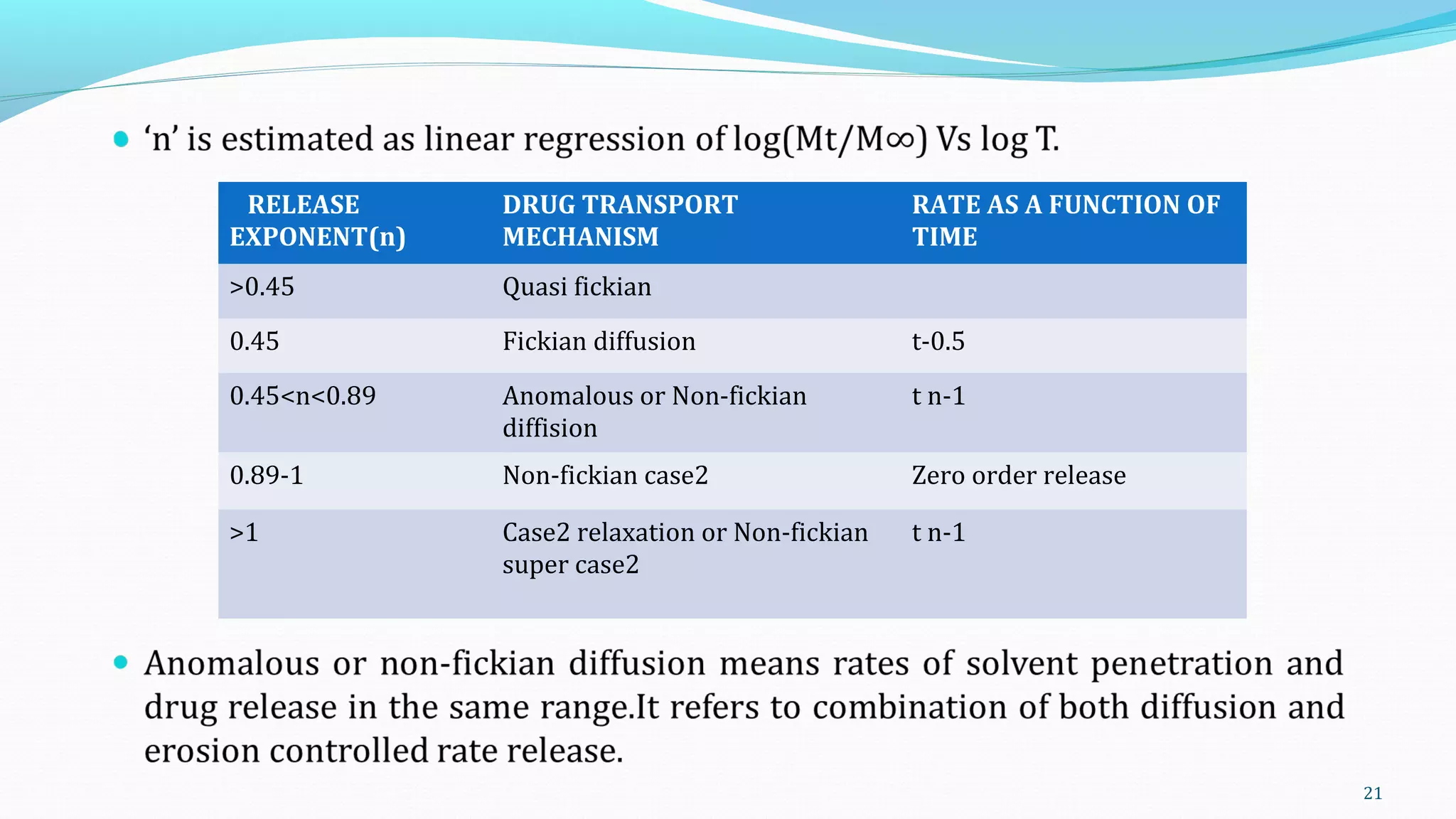
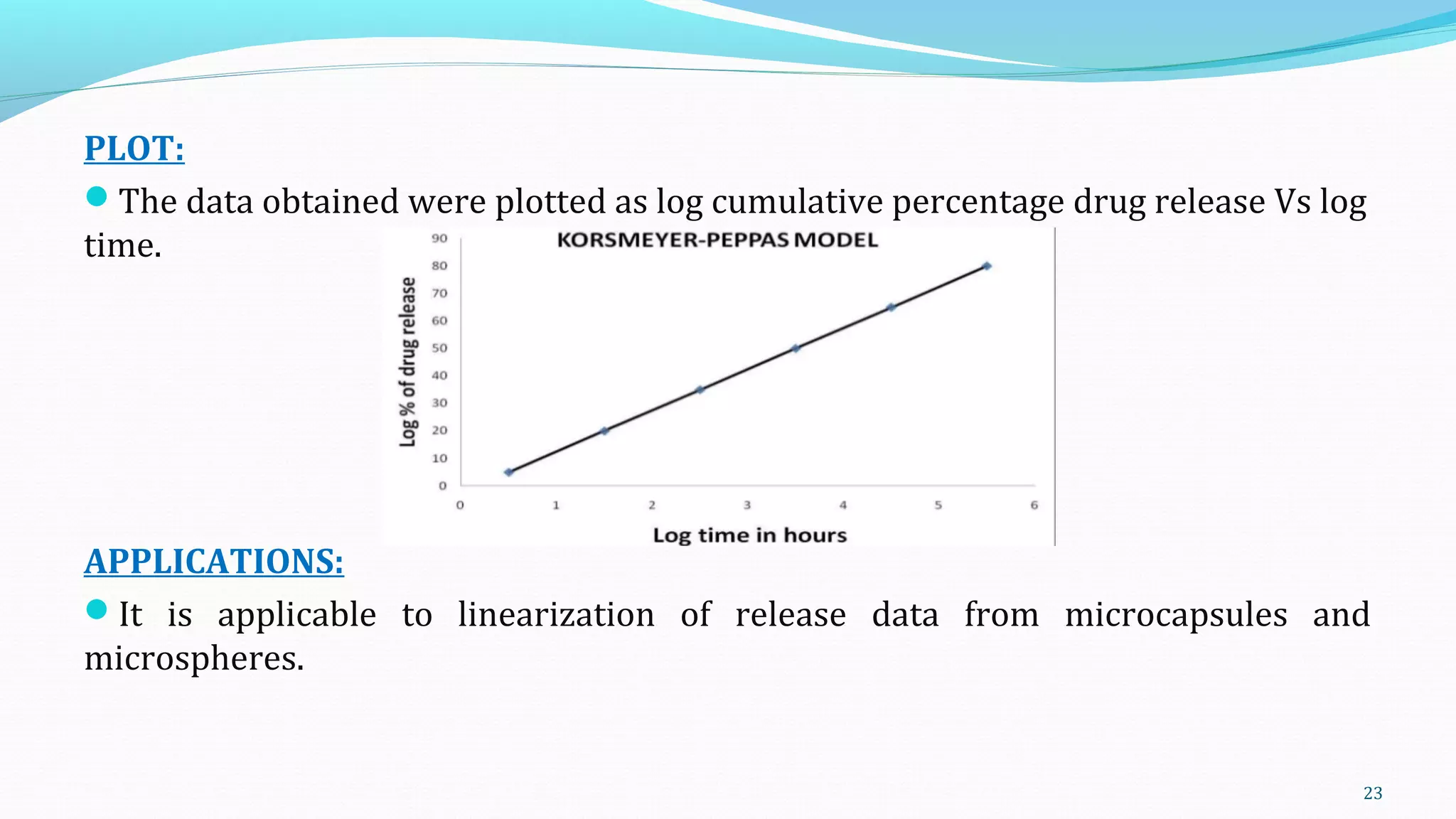
JAWAHARLAL NEHRU TECHNOLOGICAL
UNIVERSITY-KAKINADA
STUDY OF CONSOLIDATION PARAMETERS
Presented by: G.DURGA BHAVANI
M.Pharmacy 1st
yr
Pharmaceutics
18IS1S03141
CONTENTS:
HECKEL PLOTS
SIMILARITY FACTORS-F1 AND F2
HIGUCHI PLOT
PEPPAS PLOT
2
HECKEL EQUATION:
The Heckel analysis is a most popular method of deforming reduction under
pressure.
It is based upon analogous behaviour to first order reaction where the pores in
the mass are the reactant.i.e.,
Log 1/E=Ky . P+Kr
where,
Ky=material dependent constant but inversely proportional to its yield
strength(S)
Kr=related packing stage(E0)
3
4
BASED ON HECKEL EQUATION:
3 types of powders:-TYPE-A; TYPE-B; TYPE-C.
FOR TYPE-A MATERIAL:
A linear relationship is observed,with the plots remaining parallel as the
applied pressure is increased indicating deformation apparently only by plastic
deformation.
Soft materials undergo plastic deformation readily and retain different
degree of porosity,depending upon the initial packing of die. Thus, inturn
influenced by the size distribution,shape etc., of the original particals.
e.g.:-Sodium chloride
FOR TYPE-B MATERIALS:
There is an initial curved region followed by a straight line.
This indicates that the particles are fragmenting at the early stages of the
compression process.
5
Harder materials with higher yield pressure values usually undergo
compression by fragmentation first.,to provide a denser packing.
e.g:Lactose; Sucrose.
FOR TYPE-C MATERIALS:
There is an initial step linear region which become superimposed and flatten
out as applied pressure is increased.
This behavior to the absence of a rearrangement stage and densification is
due to plastic deformation and asperity melting.
Type-A plots,exhibits higher slope(Ky) than type-b,because type-a have lower
yield stress than type-a.
Type-B plots,exhibits lower slope(Ky)because brittle,hard materials are difficult
to compress.
6
7
HECKEL PLOTS:
Heckel plot is density Vs applied pressure.
It follows first order kinetics.
As porosity increases compression force also increases.
Thus,heckel plot allows for the interpretation of the mechanical bonding.
It identifies the predominent form of deformation for a given sample.
Heckel plot represent in two regions:
1.Initial repacking stage.
2.Subsequent deformation process
8
LIMITATIONS :
Heckel plot is influenced by;
1.Degree of lubrication.
2.Size of the die.
3.Residual porosity in particular formulations provide good mechanical
strength,rapid water intake and hence good disintegration characteristics.
APPLICATIONS:
Used to check lubricant efficacy.
For interpretation of consolidation mechanism.
9
MODEL INDEPENDENT METHOD:
MOORE and FLANNER propose this mathematical approach to compare
dissolution profile using 2 factors.
PAIRED WISE APPROACH:
Difference factor(F1)
Similarity factor(F2)
DIFFERENCE FACTOR(F1):
Defined by FDA i.e.,calculates the % difference between 2 curves at each
time point and is a measurement of the relative error between 2 curves.
Where;
n=no. of time points.
Rt=%dissolved at time ‘t’ of reference product(pre change).
Tt=%dissolved at time’t’ of test product(post change). 10
SIMILARITY FACTOR(F2):
Defined by FDA i.e.,Logarthemic reciprocal square root transformation of
sum of squared error and is a measurement of the similarity in the
percentage dissolution between the 2 curves.
LIMITS OF DIFFERENCE AND SIMILARITY FACTORS:
11
DATA STRUCTURE AND STEPS TO FOLLOW:
This independent model is most suitable for the dissolution profile
comparision when 3 to 4 or more dissolution time points are available.
Determine the dissolution profile of two products(12 units each) of the
test(post change)and the reference(pre change)of the products.
Using the mean dissolution values from both curves at each time
interval,calculate the difference factor and similarity factor using the above
equations.
For curves to be considered similar,F1values should be closer to ‘0’ and F2
values should be closer to 100.In general,F1 values are upto 15 (0-15) and F2
values ane greater than 50(50-100) to ensure equivalence of two curves and
thus,the performance of test and reference products.
12
SOME RECOMMENDATIONS:
The dissolution measurements of test and reference batches should be made under
exactly the same conditions.
The dissolution time profiles for both the profiles should be the same.
(e.g.,15,30,45,60 minutes)
The reference batch used should be the most recently manufactured pre change
products.
Only one measurement should be considered after 85% dissolution of both the
products(when applicable).
To allow use of mean data,for immediate release products the percent coefficient of
variation(%cv) for the individual dissolution results at the earlier time points i.e.,at
15 minutes should not be more than 20% and at the other points should not be more
than 10%.
The mean dissolution values for reference can be derived either from last pre
changed values or from last 2 or more consecutively manufactured pre change
batches. 13
CRITERIA FOR EXEMPTIONS FROM F2
COMPARISION:
When API is highly soluble across the physiologically relevant range of pH
and the dosage form exhibit very rapid dissolution.It may not be necessary to
compare the dissolution profiles.
A minimum of 3 time points(zero excluded) is generally required for the
calculation of F2 value.
It should be noted that more than 3 time points should be required to
adequately characterise the shape of the dissolution profiles.
Standard deviation of mean of any product should not be more than 10%
from 2nd
to last dissolution time point.
14
ADVANTAGES:
They are easy to compute.
They provide a single number to describe the comparison of dissolution
profile data.
DISADVANTAGES:
The values of F1 and F2 are sensitive to the no. of dissoltion time points used.
The basis of the criteria for deciding the difference or similarity between
dissolution profile is unclear.
15
APPLICATIONS:
FOR F1:
F1 is specially used to compare two dissolution profiles being necessary to
consider one of them as reference and std. Product.
It can measure the percent of error between two curves overall time points.
FOR F2:
This method is more appropriate when more than 3 or 4 dissolution time
points are available.
The F2 may became invariant with respect to location change and
consequence of failure to take into account the shape of curve and unequal
spacing between sampling time points leads to errors.
Nervertheless with the slight modification in the statistical analysis, similarity
factor would definitely serves as an efficient tool for reliable comparision of
dissolution profiles.
16
HIGUCHI MODEL:(diffusion matrix formulation)
Higuchi proposed this model in 1961 to describe drug release from matrix
system.
It is developed to study the water soluble and low soluble drugs incorporated
in semisolids and solid matrices.
It is based on the hypothesis that;
1. Initial drug concentration in the matrix is much higher than drug
solubility.
2. Drug diffusion takes place in only one direction(edge effect must be
negligible).
3. Drug particles are much smaller than system thickness.
4. Matrix swelling and dissolution are negligible.
5. Drug diffusivity is constant.
6. perfect sink conditions are always attained in the release environment
17
18
PLOT:
The data obtained were plotted as cumulative percentage drug release Vs
square root of time.
APPLICATIONS:
Modified release pharmaceutical dosage forms , transdermal systems and
matrix tablets with water soluble drugs.
19
KORSMEYER-PEPPAS MODEL:(the power law)
20
RELEASE
EXPONENT(n)
DRUG TRANSPORT
MECHANISM
RATE AS A FUNCTION OF
TIME
>0.45 Quasi fickian
0.45 Fickian diffusion t-0.5
0.45<n<0.89 Anomalous or Non-fickian
diffision
t n-1
0.89-1 Non-fickian case2 Zero order release
>1 Case2 relaxation or Non-fickian
super case2
t n-1
21
22
PLOT:
The data obtained were plotted as log cumulative percentage drug release Vs log
time.
APPLICATIONS:
It is applicable to linearization of release data from microcapsules and
microspheres.
23
CONCLUSION:
The main aim of formulation of any drug delivery system is to ensure safety
and efficacy of patients, for which study of drug release from the dosage form is
utmost important.
Thus, these mathematical models are important for prediction and elucidation
of exact behavior of drug or drug release from specific drug delivery systems.
Higuchi model has a large applications in polymeric matrix systems.
F1 and F2 comparison is easy and this is most widely used method to compare
dissolution profiles.
Hence, a single system can be explained by various models with their
comparative study and correlating outcomes of different models.
24
REFERENCES:
Hussain L,Ashwini D,Sirish D.Kinetic modeling and dissolution profiles
comparison; an overview.Int J pharm Bio Sci 2013;4(1);728-737.
The theory and practice of industrial pharmacy by Leon lachmann,
Herbert A Liberman.
Aulton’s pharmaceutics: the design and manufacture of medicines by
Micheal Aulton.
25
26

Study of consolidation parameters

  • 1.
    JAWAHARLAL NEHRU TECHNOLOGICAL UNIVERSITY-KAKINADA STUDYOF CONSOLIDATION PARAMETERS Presented by: G.DURGA BHAVANI M.Pharmacy 1st yr Pharmaceutics 18IS1S03141
  • 2.
    CONTENTS: HECKEL PLOTS SIMILARITY FACTORS-F1AND F2 HIGUCHI PLOT PEPPAS PLOT 2
  • 3.
    HECKEL EQUATION: The Heckelanalysis is a most popular method of deforming reduction under pressure. It is based upon analogous behaviour to first order reaction where the pores in the mass are the reactant.i.e., Log 1/E=Ky . P+Kr where, Ky=material dependent constant but inversely proportional to its yield strength(S) Kr=related packing stage(E0) 3
  • 4.
  • 5.
    BASED ON HECKELEQUATION: 3 types of powders:-TYPE-A; TYPE-B; TYPE-C. FOR TYPE-A MATERIAL: A linear relationship is observed,with the plots remaining parallel as the applied pressure is increased indicating deformation apparently only by plastic deformation. Soft materials undergo plastic deformation readily and retain different degree of porosity,depending upon the initial packing of die. Thus, inturn influenced by the size distribution,shape etc., of the original particals. e.g.:-Sodium chloride FOR TYPE-B MATERIALS: There is an initial curved region followed by a straight line. This indicates that the particles are fragmenting at the early stages of the compression process. 5
  • 6.
    Harder materials withhigher yield pressure values usually undergo compression by fragmentation first.,to provide a denser packing. e.g:Lactose; Sucrose. FOR TYPE-C MATERIALS: There is an initial step linear region which become superimposed and flatten out as applied pressure is increased. This behavior to the absence of a rearrangement stage and densification is due to plastic deformation and asperity melting. Type-A plots,exhibits higher slope(Ky) than type-b,because type-a have lower yield stress than type-a. Type-B plots,exhibits lower slope(Ky)because brittle,hard materials are difficult to compress. 6
  • 7.
  • 8.
    HECKEL PLOTS: Heckel plotis density Vs applied pressure. It follows first order kinetics. As porosity increases compression force also increases. Thus,heckel plot allows for the interpretation of the mechanical bonding. It identifies the predominent form of deformation for a given sample. Heckel plot represent in two regions: 1.Initial repacking stage. 2.Subsequent deformation process 8
  • 9.
    LIMITATIONS : Heckel plotis influenced by; 1.Degree of lubrication. 2.Size of the die. 3.Residual porosity in particular formulations provide good mechanical strength,rapid water intake and hence good disintegration characteristics. APPLICATIONS: Used to check lubricant efficacy. For interpretation of consolidation mechanism. 9
  • 10.
    MODEL INDEPENDENT METHOD: MOOREand FLANNER propose this mathematical approach to compare dissolution profile using 2 factors. PAIRED WISE APPROACH: Difference factor(F1) Similarity factor(F2) DIFFERENCE FACTOR(F1): Defined by FDA i.e.,calculates the % difference between 2 curves at each time point and is a measurement of the relative error between 2 curves. Where; n=no. of time points. Rt=%dissolved at time ‘t’ of reference product(pre change). Tt=%dissolved at time’t’ of test product(post change). 10
  • 11.
    SIMILARITY FACTOR(F2): Defined byFDA i.e.,Logarthemic reciprocal square root transformation of sum of squared error and is a measurement of the similarity in the percentage dissolution between the 2 curves. LIMITS OF DIFFERENCE AND SIMILARITY FACTORS: 11
  • 12.
    DATA STRUCTURE ANDSTEPS TO FOLLOW: This independent model is most suitable for the dissolution profile comparision when 3 to 4 or more dissolution time points are available. Determine the dissolution profile of two products(12 units each) of the test(post change)and the reference(pre change)of the products. Using the mean dissolution values from both curves at each time interval,calculate the difference factor and similarity factor using the above equations. For curves to be considered similar,F1values should be closer to ‘0’ and F2 values should be closer to 100.In general,F1 values are upto 15 (0-15) and F2 values ane greater than 50(50-100) to ensure equivalence of two curves and thus,the performance of test and reference products. 12
  • 13.
    SOME RECOMMENDATIONS: The dissolutionmeasurements of test and reference batches should be made under exactly the same conditions. The dissolution time profiles for both the profiles should be the same. (e.g.,15,30,45,60 minutes) The reference batch used should be the most recently manufactured pre change products. Only one measurement should be considered after 85% dissolution of both the products(when applicable). To allow use of mean data,for immediate release products the percent coefficient of variation(%cv) for the individual dissolution results at the earlier time points i.e.,at 15 minutes should not be more than 20% and at the other points should not be more than 10%. The mean dissolution values for reference can be derived either from last pre changed values or from last 2 or more consecutively manufactured pre change batches. 13
  • 14.
    CRITERIA FOR EXEMPTIONSFROM F2 COMPARISION: When API is highly soluble across the physiologically relevant range of pH and the dosage form exhibit very rapid dissolution.It may not be necessary to compare the dissolution profiles. A minimum of 3 time points(zero excluded) is generally required for the calculation of F2 value. It should be noted that more than 3 time points should be required to adequately characterise the shape of the dissolution profiles. Standard deviation of mean of any product should not be more than 10% from 2nd to last dissolution time point. 14
  • 15.
    ADVANTAGES: They are easyto compute. They provide a single number to describe the comparison of dissolution profile data. DISADVANTAGES: The values of F1 and F2 are sensitive to the no. of dissoltion time points used. The basis of the criteria for deciding the difference or similarity between dissolution profile is unclear. 15
  • 16.
    APPLICATIONS: FOR F1: F1 isspecially used to compare two dissolution profiles being necessary to consider one of them as reference and std. Product. It can measure the percent of error between two curves overall time points. FOR F2: This method is more appropriate when more than 3 or 4 dissolution time points are available. The F2 may became invariant with respect to location change and consequence of failure to take into account the shape of curve and unequal spacing between sampling time points leads to errors. Nervertheless with the slight modification in the statistical analysis, similarity factor would definitely serves as an efficient tool for reliable comparision of dissolution profiles. 16
  • 17.
    HIGUCHI MODEL:(diffusion matrixformulation) Higuchi proposed this model in 1961 to describe drug release from matrix system. It is developed to study the water soluble and low soluble drugs incorporated in semisolids and solid matrices. It is based on the hypothesis that; 1. Initial drug concentration in the matrix is much higher than drug solubility. 2. Drug diffusion takes place in only one direction(edge effect must be negligible). 3. Drug particles are much smaller than system thickness. 4. Matrix swelling and dissolution are negligible. 5. Drug diffusivity is constant. 6. perfect sink conditions are always attained in the release environment 17
  • 18.
  • 19.
    PLOT: The data obtainedwere plotted as cumulative percentage drug release Vs square root of time. APPLICATIONS: Modified release pharmaceutical dosage forms , transdermal systems and matrix tablets with water soluble drugs. 19
  • 20.
  • 21.
    RELEASE EXPONENT(n) DRUG TRANSPORT MECHANISM RATE ASA FUNCTION OF TIME >0.45 Quasi fickian 0.45 Fickian diffusion t-0.5 0.45<n<0.89 Anomalous or Non-fickian diffision t n-1 0.89-1 Non-fickian case2 Zero order release >1 Case2 relaxation or Non-fickian super case2 t n-1 21
  • 22.
  • 23.
    PLOT: The data obtainedwere plotted as log cumulative percentage drug release Vs log time. APPLICATIONS: It is applicable to linearization of release data from microcapsules and microspheres. 23
  • 24.
    CONCLUSION: The main aimof formulation of any drug delivery system is to ensure safety and efficacy of patients, for which study of drug release from the dosage form is utmost important. Thus, these mathematical models are important for prediction and elucidation of exact behavior of drug or drug release from specific drug delivery systems. Higuchi model has a large applications in polymeric matrix systems. F1 and F2 comparison is easy and this is most widely used method to compare dissolution profiles. Hence, a single system can be explained by various models with their comparative study and correlating outcomes of different models. 24
  • 25.
    REFERENCES: Hussain L,Ashwini D,SirishD.Kinetic modeling and dissolution profiles comparison; an overview.Int J pharm Bio Sci 2013;4(1);728-737. The theory and practice of industrial pharmacy by Leon lachmann, Herbert A Liberman. Aulton’s pharmaceutics: the design and manufacture of medicines by Micheal Aulton. 25
  • 26.