STATISTICALMODELING IN PHARMACEUTICAL
RESEARCHAND DEVELOPMENT
1
CONTENTS
 Statistical Modeling
 Descriptive Versus Mechanistic Modeling
 Statistical Parameters Estimation
 Confidence Regions
 Non Linearity at the Optimum
 Sensitivity Analysis
 Optimal Design
 Population Modeling
 References
2
Statistical Modeling
 The new major challenge that the pharmaceutical industry is facing in the discovery and development
of new drugs is to reduce the costs and time needed from discovery to market, while at the same
time raising standards of quality.
 If the pharmaceutical industry cannot find a solution to reduce both costs and time , then its whole
business model will be jeopardized.
 The market will hardly be able , even in the near future , to afford excessively expensive drugs,
regardless of their quality .
4
 In parallel to this growing challenge , technologies are also dramatically evolving , opening doors to
opportunities never seen before.
 This standard way to discover new drugs is essentially by trial and error .
 The “new technologies “ approach has given rise to new hope in that it has permitted many more
attempts per unit time , increasing proportionally , however , also the number of errors .
 The development of models in the pharmaceutical industry is certainly one of the significant
breakthroughs proposed to face the challenges of cost , speed , and quality , somewhat imitating
what happens in the aeronautics industry.
 The concept, however , is that of adapting just another new technology , known as modelling 5
Objectives
 The use of models in the experimental cycle to reduce cost and time and improve quality .
 Without models , the final purpose of an experiment was one single drug or its behavior . With the
use of models , the objective of experiment will be the drug and the models at the same level.
 Improving the models will help understanding the experiment on successive drugs and improving
the model’s ability will help to represent reality.
6
Concept
 According to breiman , there are two cultures in the use of statistical modelling to reach conclusions
from data.
 The first culture , namely , the data modelling culture , assumes that the data are
generated by a given stochastic data model.
 Whereas the other , the algorithmic modelling culture , uses algorithmic models and
treats the data mechanism as unknown.
 To understand the mechanism , the use of modeling concepts is essential.
 Statistics thinks of the data as being generated by a black box into which a vector of input variables x
(independent variable) enter and out of which a vector of response variables y (dependent variable)
exits.
7
Contd..,
 The purpose of the model is essentially for that of translating the known properties about the black
box as well as some new hypotheses into a mathematical representation.
 In this way , a model is a simplifying representation of the data – generating mechanism under
investigation.
 The identification of an appropriate model is often not easy and may require thorough investigation.
8
Contd..,
 Two of the main goals of performing statistical investigations are to be able to predict,
 what the responses are going to be future input variables
 To Extract some information about how nature is associating the response variables to the
input variables.
 A third possible goal might be
 To understand the foundations of the mechanisms from which the data are generated or going
to be generated.
9
Descriptive versus mechanistic modeling
Descriptive model:
 In this type of model, the purpose is to provide a reasonable description of the data in some
appropriate way without any attempt at understanding the underlying phenomenon , that is the
data-generating mechanism , then the family of models is selected based on its adequacy to
represents the data structure
 In this instance, the order of the model is chosen based on its competence to describe the data
arrangement.
 This type of model is very useful for discriminating between alternating hypothesis but are useless
for capturing the fundamental characteristics of a mechanism.
Mechanistic model:
 In the mechanistic model, the importance rests in the knowledge of the device of development, it
is important to be able to score on a powerful collaboration among scientists, specialists in the
field and statisticians or mathematicians.
 The former must provide updated , rich and reliable information about the problem.
 whereas the latter are trained for translating scientific information in mathematical models.
Purpose of the module :
 To translate the known properties about as well as some new hypothesis into a mathematical
representation.
 The family of models is selected depends on the main purpose of the exercise.
 If the purpose is just to provide a reasonable description of the data without any attempt at
understanding the underlying phenomenon, that is, the data-generating mechanism.
 Then the family of models is selected based on its adequacy to represent the data structure.
13
 Animal tumor growth data are used for the representation of the different concepts encountered
during the development of a model and its after-identification use.
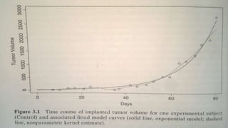
 The data represent the tumor growth in rats over a period of 80 days.
 We are interested in modeling the growth of experimental tumors subcutaneously implanted in rats
to be able to differentiate between treatment regimens.
14
 Two groups of rats have received different treatments, placebo and a new drug at a fixed dose.
 So in addition to the construction of an appropriate model for representing the tumor growth, there
is an interest in the statistical significance of the effect of treatment .
 The raw data for one subject who received placebo are represented as open circles. For the
considered subject, the tumor volume grows from nearly 0 to about 3000 cubic millimeter.
15
 A first evaluation of the data can be done by running nonparametric statistical estimation techniques
like, for example, the Nadaraya–Watson kernel regression estimate.
 These techniques have the advantage of being relatively cost-free in terms of assumptions, but they
do not provide any possibility of interpreting the outcome and are not at all reliable when
extrapolating.
 These techniques attempt to optimize the selection of the parameter value with respect to a certain
criterion.
 The ordinary least-squares optimization algorithm has been used to get parameter estimates.
16
Example 1
 The special characteristics of the growth curves are that the exhibited growth profile generally is a
nonlinear function of time with an asymptote;
 That random variability associated to the data is likely to increase with size, so that the dispersion is
not constant;
 And finally, that successive responses are measured on the same subject so that they will generally
not be independent .
 Note that different individuals may have different tumor growth rates, either inherently or because of
environmental effects or treatment.
17
18
 The growth rate of a living organism or tissue can often be characterized by two competing
processes.
 The net increase is then given by the difference between anabolism and catabolism, between the
synthesis of new body matter and its loss.
 Catabolism is often assumed to be proportional to the quantity chosen to characterize the size of the
living being, namely, weight or volume, where as anabolism is assumed to have an allometric
relationship to the same quantity.
19
Example 2
 These assumptions on the competing processes are translated into mathematics by the following
differential equation
 where µ(t) represents size of studied system in function of time
20
 Note that this equation can be reformulated as follows:
 which has μ(t) = α(1 + K exp(–γ(t – η)–1/K as general solution.
 The curve represented by this last equation is commonly named the Richards curve.
 When K is equal to one, the Richards curve becomes the well-known logistic function.
 If the allometric factor in the relationship representing the catabolism mechanism is small, that is, K tends to 0,
then the different equation becomes :
21
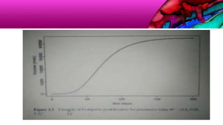
 The different curves obtained by increasing the number of terms in the Taylor expansion are
represented in Gompertz curve itself.
 The exponential growth model can thus be now justified not only because it fits well the data but
also because it can be seen as a first approximation to the Gompertz growth model, which is
endowed with a mechanistic interpretation , namely, competition between the catabolic and anabolic
processes. 22
Statistical parameters estimation
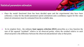
 Once the model functional form has been decided upon and the experimental data have been
collected, a value for the model parameters (point estimation) and a confidence region for this value
(interval estimation) must be estimated from the available data.
 In its simplest form , the ordinary least squares criterion (OLS) prescribes as a loss function the
sum of the squared “residuals” relative to all observed points, where the residual relative to each
observed point is the difference between the observed and predicted value at that point.
25
Approximations of the Gompertz growth curve based on Taylor expansion
for the internal exponential term.
26
 Clearly, if the model resulting from a certain parameter value tends to closely predict the actually
observed values, then the residuals will be small and the sum of their squares will also be small, so
the loss will be small.
 Conversely, a bad or unacceptable value of the parameter will determine a model that predicts values
very far from those actually observed, the residuals will be large and the loss will be large.
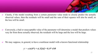
 We may suppose, in general, to have a nonlinear model with a known functional relationship
yi = u(xi;θ*) + εi, E[εi] = 0, θ* ∈ Θ
27
 where yi is the ith observation, corresponding to a vector xi of independent variables, where θ* is
the true but unknown parameter value belonging to some acceptable domain Θ,
 where u is the predicted value as a function of independent variables and parameter, and where εi
are true errors (which we only suppose for the moment to have zero mean value) that randomly
modify the theoretical value of the observation.
 We may rewrite the model in vector form as
y = u(X, θ*) + ε, E[ε] = 0, θ* ∈ Θ.
28
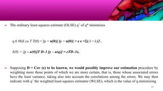
 The ordinary least-squares estimate (OLSE) qˆ of q* minimizes
q ∈ Θ)S yu T T(θ) = [y − u(θ)] [y − u(θ)] = e e =Σ( i − i )2 .
S(θ) = [y – u(θ)]T D–1 [y – u(q)] = eTD–1e,
 Supposing D = Cov (e) to be known, we would possibly improve our estimation procedure by
weighting more those points of which we are more certain, that is, those whose associated errors
have the least variance, taking also into account the correlations among the errors. We may then
indicate with qˆ the weighted least-squares estimator (WLSE), which is the value of q minimizing
29
S(θ) = [y – u(θ)]T D–1 [y – u(θ)] = eTD–1e,
 where e is the vector of “residuals” [y − u(q)].
 In the case in which the errors are independent of each other their co variances will be zero, and if
they also have the same variance,
 then D = σ2I,with the constant σ2 being the common variance
 Typically, either a simplex algorithm (which does not require or depend on the numerical
computation of derivatives of the loss with respect to the parameters) or a more efficient, derivative-
based nonlinear non constrained quasi-Newton variable metric optimization algorithm may be used
with a stopping criterion based on the convergence of either loss function or parameter value. 30
CONFIDENCE REGIONS
 In statistics, a confidence region is a multi-dimensional generalization of a confidence interval. It
is a set of points in an n-dimensional space, often represented as an ellipsoid around a point which
is an estimated solution to a problem, although other shapes can occur.
Interpretation:
 The confidence region is calculated in such a way that if a set of measurements were repeated many
times and a confidence region calculated in the same way on each set of measurements, then a
certain percentage of the time (e.g. 95%) the confidence region would include the point
representing the "true" values of the set of variables being estimated.
 However, unless certain assumptions about prior probabilities are made, it does not mean, when
one confidence region has been calculated, that there is a 95% probability that the "true" values lie
inside the region, since we do not assume any particular probability distribution of the "true" values
and we may or may not have other information about where they are likely to lie.
CONFIDENCE REGIONS
 Suppose D = Cov(e), known. Indicate with θqˆ the weighted least-squares estimator (WLSE),
that is, let θ minimize
S(θ) = [y – u(q)]T D-1[y-u(θ) [y – u(θ)] =eTD–1e.
 Expanding u in Taylor series around the true q* and neglecting terms of second and higher
order we may write
33
34
If we believe that
D = σ2 diag(u)
that is, that errors are independent and proportional to the square root of the predicted value, then
D–1 =diag(1/ui)/σ2,
 where we may further approximate this result by estimating
 A first approach to the definition of the confidence regions in parameter space follows the
linear approximation to the parameter joint distribution that we have already used: If the
estimates are approximately normally distributed around
35
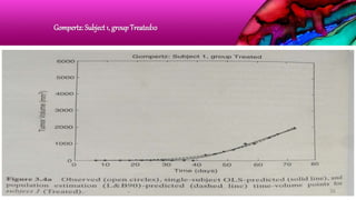
Gompertz: Subject 1, group Treated10
36
Gompertz: Subject 4, group Treated
37
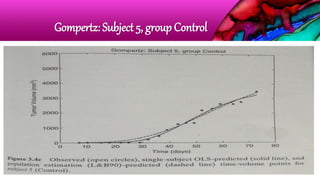
Gompertz: Subject 5, group Control
38
Gompertz: Subject 8, group Control
39
Nonlinearity at the optimum
Nonlinearity at the optimum:
 The problem now is that of deciding that this indeed the case. To this end it is useful to study the
degree of non linearity of our module in a neighborhood of the forecast.
 We refer the reader to the general treatment by seber and wild, relating essentially work of bates and
watts.
 Briefly, there exist method of assessing the maximum degree of intrinsic nonlinearity is excessive ,
for one or more parameters the confidence regions obtained applying the results of the classic theory
are not to be trusted .
 In this case, alternative simulation procedure may be employed to provide empirical confidence
region.
41
SENSITIVITY ANAYSIS
 Sensitivity analysis is the study of how the uncertainty in the output of a mathematical model or
system (numerical or otherwise) can be divided and allocated to different sources of uncertainty in
its inputs.
 A related practice is uncertainty analysis, which has a greater focus on uncertainty quantification
and propagation of uncertainty; ideally, uncertainty and sensitivity analysis should be run in
tandem.
 The process of recalculating outcomes under alternative assumptions to determine the impact of a
variable under sensitivity analysis can be useful for a range of purposes, including:
• Testing the robustness of the results of a model or system in the presence of
uncertainty.
• Increased understanding of the relationships between input and output
variables in a system or model.
SENSITIVITY ANAYSIS:
• Uncertainty reduction, through the identification of model inputs that cause significant
uncertainty in the output and should therefore be the focus of attention in order to increase
robustness (perhaps by further research).
• Searching for errors in the model (by encountering unexpected relationships between
inputs and outputs).
• Model simplification – fixing model inputs that have no effect on the output, or identifying
and removing redundant parts of the model structure.
• Enhancing communication from modelers to decision makers (e.g. by making
recommendations more credible, understandable, compelling or persuasive).
• Finding regions in the space of input factors for which the model output is either maximum
or minimum or meets some optimum criterion (see optimization and Monte Carlo
filtering).
• In case of calibrating models with large number of parameters, a primary sensitivity test
can ease the calibration stage by focusing on the sensitive parameters. Not knowing the
sensitivity of parameters can result in time being uselessly spent on non-sensitive ones.
• To seek to identify important connections between observations, model inputs, and
predictions or forecasts, leading to the development of better models
 The choice of method of sensitivity analysis is typically dictated by a number of problem constraints
or settings. Some of the most common are
• Computational expense
• Correlated inputs
• Nonlinearity
• Model interactions
• Multiple outputs
• Given data
Sensitivity analysis methods:
 There are a large number of approaches to performing a sensitivity analysis, many of which have
been developed to address one or more of the constraints discussed above.[2] They are also
distinguished by the type of sensitivity measure, be it based on (for example) variance
decompositions, partial derivatives or elementary effects.
 Derivative-based local method
 Regression analysis
 Variance-based methods
 Variogram analysis of response surfaces (VARS)
 Screening
Derivative-based local method:
 Local derivative-based methods involve taking the partial derivative of the output Y with respect
to an input factor Xi
Regression analysis:
 Regression analysis, in the context of sensitivity analysis, involves fitting a linear regression to
the model response and using standardized regression coefficients as direct measures of
sensitivity. The regression is required to be linear with respect to the data (i.e. a hyperplane,
hence with no quadratic terms, etc., as regressors) because otherwise it is difficult to interpret the
standardised coefficients. This method is therefore most suitable when the model response is in
fact linear; linearity can be confirmed, for instance, if the coefficient of determination is large.
The advantages of regression analysis are that it is simple and has a low computational cost
Variance-based methods:
 Variance-based methods are a class of probabilistic approaches which quantify the input
and output uncertainties as probability distributions, and decompose the output variance into
parts attributable to input variables and combinations of variables. The sensitivity of the
output to an input variable is therefore measured by the amount of variance in the output
caused by that input
Variogram analysis of response surfaces (VARS):
 One of the major shortcomings of the previous sensitivity analysis methods is that none of
them considers the spatially ordered structure of the response surface/output of the model
Y=f(X) in the parameter space.
 Accordingly, in the VARS framework, the values of directional variograms for a given
perturbation scale can be considered as a comprehensive illustration of sensitivity
information, through linking variogram analysis to both direction and perturbation scale
concepts. As a result, the VARS framework accounts for the fact that sensitivity is a scale-
dependent concept, and thus overcomes the scale issue of traditional sensitivity analysis
methods
Screening
 Screening is a particular instance of a sampling-based method. The objective here is rather
to identify which input variables are contributing significantly to the output uncertainty in
high-dimensionality models, rather than exactly quantifying sensitivity (i.e. in terms of
variance). Screening tends to have a relatively low computational cost when compared to
other approaches, and can be used in a preliminary analysis to weed out uninfluential
variables before applying a more informative analysis to the remaining set. One of the most
commonly used screening method is the elementary effect method
SENSITIVITYANAYSISCONTD,….
 The goal here is to determine the (relative) effect of a variation in a given parameter value on the
model prediction. Let y= u(X, q) + e be the considered model, with y ∈ Δm and q ∈ Θ ⊂ Δq
 The sensitivity of the modeling function u with respect to the parameter q by means of the
(absolute) sensitivity coefficient, which is the partial derivative.
 Means of the normalized sensitivity coefficient
 The normalization serves to make sensitivities comparable across variables and parameters.
51
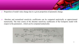
 Proportion of model value change due to a given proportion of parameter change.
 Absolute and normalized sensitivity coefficients can be computed analytically or approximated
numerically. The time course of the absolute sensitivity coefficients of the Gompertz model with
respect to the parameters , which can be computed analytically:
52
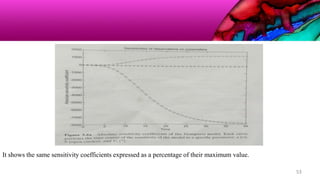
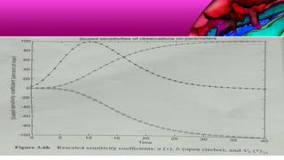
It shows the same sensitivity coefficients expressed as a percentage of their maximum value.
53
54
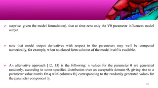
 surprise, given the model formulation), that at time zero only the V0 parameter influences model
output.
 note that model output derivatives with respect to the parameters may well be computed
numerically, for example, when no closed form solution of the model itself is available.
 An alternative approach [12, 13] is the following: n values for the parameter θ are generated
randomly, according to some specified distribution over an acceptable domain Θ, giving rise to a
parameter value matrix Θn.q with columns Θ.j corresponding to the randomly generated values for
the parameter component θj.
55
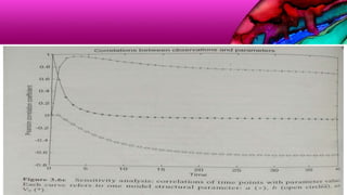
 The higher the importance of variations of θj in producing variations of uk.
 Figure 3.6c shows the time course of the Pearson MCCC between V and the three model parameters
for such a Monte Carlo simulation with n = 10,000, having generated values for the three parameters
out of uniform distributions respectively on the intervals [0.9, 1.1],
 The main advantage of this scheme is that the required number of samples does not grow as fast as a
regular Monte Carlo sampling from the joint distribution of the parameters as the number of
parameters increases.
56
57
 The influence of parameter a on tumor size, as judged from classic sensitivity analysis, seems to
increase monotonically to a plateau, reaching about 50% of its effect no sooner than day 13;
 Conversely, MCCC indicates a fast increase of effect of parameter a up to a peak at about day 3 or 4,
with a subsequent decrease and attainment of the plateau from above.
 From the sensitivity diagrams it would appear that the influence of parameterV0 is small at the
beginning, peaks over the range approximately between8 and 12 days, and slowly fades, being still
evident at 20 days; conversely, the MCCC study would indicate its maximal effect at the very
beginning of the experiment, with a subsequent fast monotonic decrease to essentially zero within 5
days.
58
 The qualitative differences of the behavior of parameter b under sensitivity or MCCC analyses are
less obvious, even if its (negative) influence on volume size seems to increase faster according to
MCCC.
 In the described MC simulation, the action of several simultaneous sources of variation is considered.

 The explanation of the different time courses of parameter influence on volume size between
sensitivity and MCCC analyses lies in the fact that classic sensitivity analysis considers variations in
model output due exclusively to the variation of one parameter component at a time, all else being
equal. In these conditions, the regression coefficient between model output and parameter component
value, in a small interval around the considered parameter, is approximately equal to the partial
derivative of the model output with respect to the parameter component. 59
Optimal design
 In the design of experiments, optimal designs (or optimum designs) are a class of experimental
designs that are optimal with respect to some statistical criterion. The creation of this field of
statistics has been credited to Danish statistician Kirstine Smith.
 In the design of experiments for estimating statistical models, optimal designs allow parameters to
be estimated without bias and with minimum variance. A non-optimal design requires a greater
number of experimental runs to estimate the parameters with the same precision as an optimal
design. In practical terms, optimal experiments can reduce the costs of experimentation.
 The optimality of a design depends on the statistical model and is assessed with respect to a
statistical criterion, which is related to the variance-matrix of the estimator. Specifying an
appropriate model and specifying a suitable criterion function both require understanding of
statistical theory and practical knowledge with designing experiments.
Optimal design
 Several design optimization criteria exist, the obvious approach is to choose the time points so as to
minimize the parameter estimate dispersion (variance-covariance) matrix, which in our case, for
ordinary least squares estimation, is approximated by the inverse of the Fisher information matrix
(FIM) at the optimum.
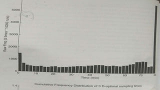
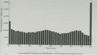
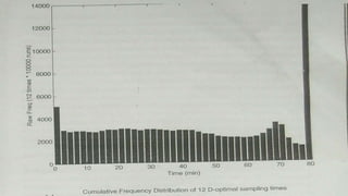
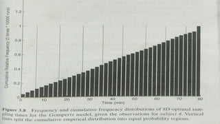
 This last method, called D-optimal design (D as in determinant) is possibly the most widely utilized
method of optimal design to find optimal sampling times for either a three-sample , an eight-sample,
or a twelve-sample experiment.
 The key idea is to obtain a large artificial sample of values of the parameter appropriately distributed
and for each value of the parameter to maximize the determinant of the FIM with respect to the
choice of times. 62
 To each such parameter value there will correspond therefore a choice of 3 (or 8 or 12) sampling
times that will maximize the FIM under the hypothesis that the parameter value is actually equal to
the one considered.
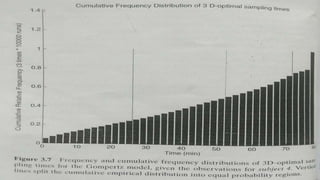
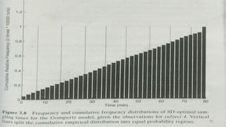
 Then build a histogram showing the frequency with which sampling times have been chosen as
optimal and use this empirical distribution of optimal sampling times to pick the times that we
consider most appropriate for the next experiments.
 The above strategy using the observations from subject 4 as our pilot sample. Report the obtained
frequency distributions of sampling times for 3, 8, and 12 sampling times, respectively , as well as
their cumulative distributions.
63
A-optimality ("average" or trace) :
 One criterion is A-optimality, which seeks to minimize the trace of the inverse of the information matrix. This
criterion results in minimizing the average variance of the estimates of the regression coefficients.
C-optimality :
 This criterion minimizes the variance of a best linear unbiased estimator of a predetermined linear
combination of model parameters.
D-optimality (determinant) :
 A popular criterion is D-optimality, which seeks to minimize |(X'X)−1|, or equivalently maximize the
determinant of the information matrix X'X of the design. This criterion results in maximizing the differential
Shannon information content of the parameter estimates.
E-optimality (eigenvalue) :
 Another design is E-optimality, which maximizes the minimum eigenvalue of the information matrix.
T-optimality :
 This criterion maximizes the trace of the information matrix. Other optimality-criteria are concerned
with the variance of predictions
G-optimality:
 A popular criterion is G-optimality, which seeks to minimize the maximum entry in the diagonal of
the hat matrix X(X'X)−1X'. This has the effect of minimizing the maximum variance of the predicted
values.
I-optimality (integrated):
 A second criterion on prediction variance is I-optimality, which seeks to minimize the average
prediction variance over the design space.
V-optimality (variance):
 A third criterion on prediction variance is V-optimality, which seeks to minimize the average
prediction variance over a set of m specific points.
Optimal designs offer three advantages over sub-optimal experimental designs:
 Optimal designs reduce the costs of experimentation by allowing statistical models to be estimated
with fewer experimental runs.
 Optimal designs can accommodate multiple types of factors, such as process, mixture, and discrete
factors.
 Designs can be optimized when the design-space is constrained, for example, when the
mathematical process-space contains factor-settings that are practically infeasible (e.g. due to safety
concerns).
advantages of Optimal design
67
68
69
70
71
72
Population Modeling
Population Modeling
 A population model is a type of mathematical model that is applied to the study of population
dynamics.
 The standard way to proceed would be to fit the model to the data relative to each experimental unit,
one at a time, thus obtaining a sample of parameter estimates, one for each experimental tumor
observed.
 The sample mean and dispersion of these estimates would then constitute our estimate of the
population mean and dispersion.
 By the same token, we could find the mean and dispersion in the “Control” and “Treated” subsamples.
74
 Population pharmacokinetic (PK) modeling involves estimating an unknown population
distribution based on data from a collection of nonlinear models.
 A drug is given to a population of subjects. In each subject, the drug’s behavior is stochastically
described by an unknown subject-specific parameter vector ∂.
 This vector ∂ varies significantly (often genetically) between subjects, which accounts for the
variability of the drug response in the population.
 The mathematical problem is to determine the population parameter distribution F (∂) based on the
clinical data
 There are two problems with the above procedure, however. The first is that it is not efficient,
because the inter subject parameter variance it computes is actually the variance of the parameters
between subjects plus the variance of the estimate of a single-subject parameter.
 The second drawback is that often, in real-life applications, a complete data set, with sufficiently
many points to reliably estimate all model parameters, is not available for each experimental subject.
Rationale:
 Models allow a better understanding of how complex interactions and processes work. Modeling of
dynamic interactions in nature can provide a manageable way of understanding how numbers
change over time or in relation to each other. Many patterns can be noticed by using population
modeling as a tool. 76
The Components of
PopulationModels:
 Population modeling requires accurate information on dosing, measurements, and covariates.
 Population models are comprised of several components:
• structural models,
• stochastic models, and
• covariate models.
Structural models :
 Structural models are functions that describe the time course of a measured response, and can be represented
as algebraic or differential equations.
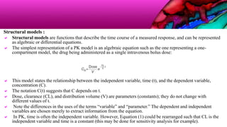
 The simplest representation of a PK model is an algebraic equation such as the one representing a one-
compartment model, the drug being administered as a single intravenous bolus dose:
 This model states the relationship between the independent variable, time (t), and the dependent variable,
concentration (C).
 The notation C(t) suggests that C depends on t.
 Dose, clearance (CL), and distribution volume (V) are parameters (constants); they do not change with
different values of t.
 Note the differences in the uses of the terms “variable” and “parameter.” The dependent and independent
variables are chosen merely to extract information from the equation.
 In PK, time is often the independent variable. However, Equation (1) could be rearranged such that CL is the
independent variable and time is a constant (this may be done for sensitivity analysis for example).
Stochastic models :
 Stochastic models describe the variability or random effects in the observed data.
 Population models provide a means of characterizing the extent of between-subject (e.g., the
differences in exposure between one patient and another) and between-occasion variability (e.g., the
differences in the same patient from one dose to the next) that a drug exhibits for a specific dose
regimen in a particular patient population.
 Variability is an important concept in the development of safe and efficacious dosing; if a drug has a
relatively narrow therapeutic window but extensive variability, then the probability of both
subtherapeutic and/or toxic exposure may be higher,24 making the quantitation of variability an
important objective for population modeling.
covariate models:
 covariate models describe the influence of factors such as demographics or disease on the individual
time course of the response.
 Describe the influence of factors such as demographics or disease on the individual time course of
the response.
 The identification of covariates that explain variability is an important objective of any population
modeling evaluation.
 During drug development, questions such as “how much does drug exposure vary with age?” are
often answered by the results of clinical trials in healthy young and elderly subjects.
 However, such information can also be garnered through population modeling.
 Population modeling develops quantitative relationships between covariates (such as age) and
parameters, accounting for “explainable” BSV by incorporating the influence of covariates on
THETA.
References:
 Computers in Pharmaceutical Research and Development
By Wiley
81
Statistical modeling in pharmaceutical research and development