Download to read offline
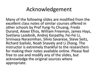


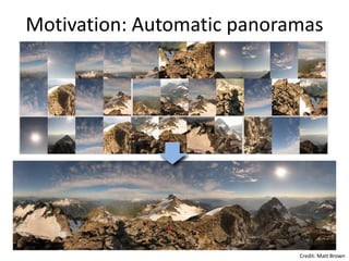


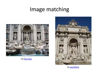
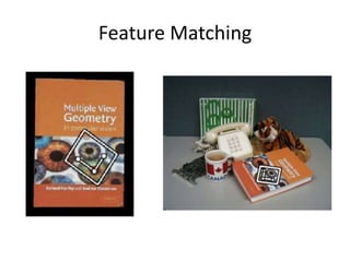

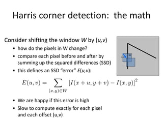
![Local features: main components
1) Detection: Identify the interest
points
2) Description: Extract vector
feature descriptor surrounding
each interest point.
3) Matching: Determine
correspondence between
descriptors in two views
],,[ )1()1(
11 dxx x
],,[ )2()2(
12 dxx x
Kristen Grauman](https://image.slidesharecdn.com/lec04harris-200719135038/85/Computer-Vision-harris-30-320.jpg)


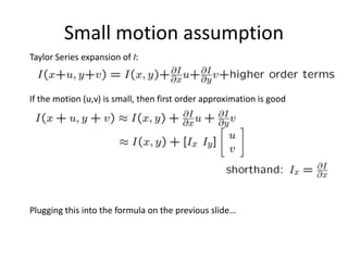
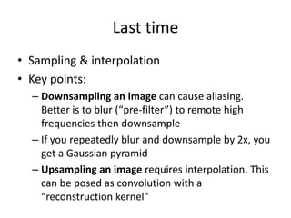
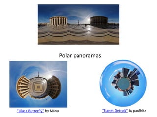
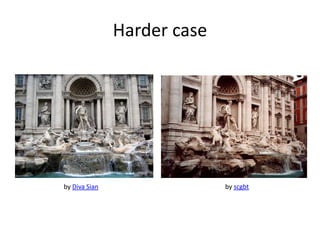
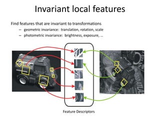
![General case
We can visualize H as an ellipse with axis lengths
determined by the eigenvalues of H and orientation
determined by the eigenvectors of H
direction of the
slowest change
direction of the
fastest change
(max)-1/2
(min)-1/2
const][
v
u
Hvu
Ellipse equation:
max, min : eigenvalues of H](https://image.slidesharecdn.com/lec04harris-200719135038/85/Computer-Vision-harris-43-320.jpg)
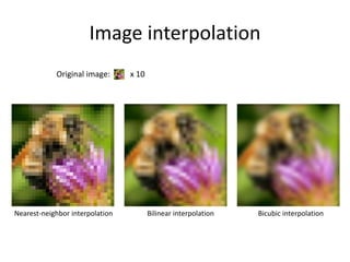
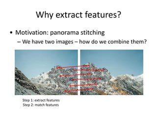
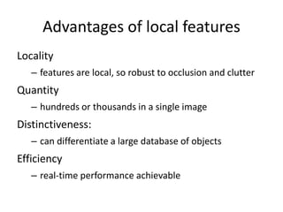
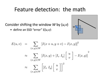
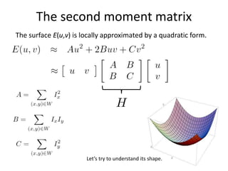
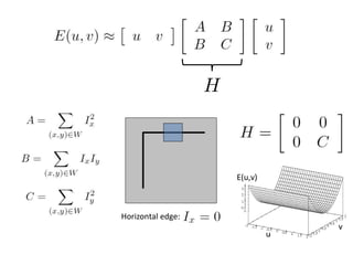
![The surface E(u,v) is locally approximated by a quadratic form.
The second moment matrix
v
u
MvuvuE ][),(
2
2
yyx
yxx
III
III
M](https://image.slidesharecdn.com/lec04harris-200719135038/85/Computer-Vision-harris-44-320.jpg)
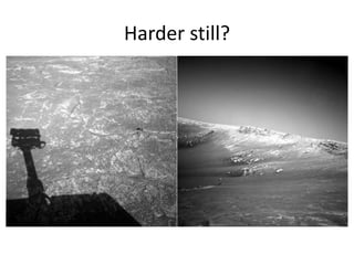
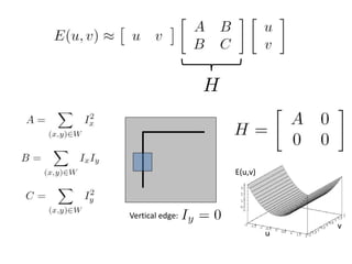
![The surface E(u,v) is locally approximated by a quadratic form. Let’s try to
understand its shape.
Interpreting the second moment matrix
v
u
HvuvuE ][),(
2
2
yyx
yxx
III
III
H](https://image.slidesharecdn.com/lec04harris-200719135038/85/Computer-Vision-harris-47-320.jpg)
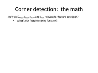
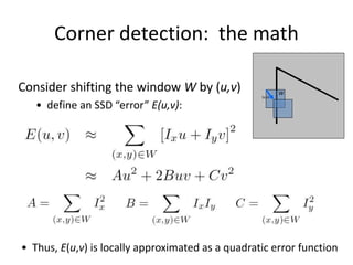
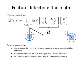
![Corner detection: the math
How are max, xmax, min, and xmin relevant for feature detection?
• What’s our feature scoring function?
Want E(u,v) to be large for small shifts in all directions
• the minimum of E(u,v) should be large, over all unit vectors [u v]
• this minimum is given by the smaller eigenvalue (min) of H](https://image.slidesharecdn.com/lec04harris-200719135038/85/Computer-Vision-harris-51-320.jpg)
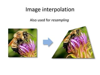
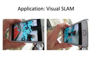
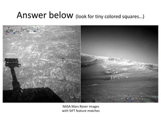
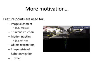
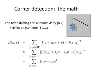
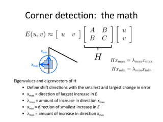
![Harris Detector [Harris88]
• Second moment matrix
)()(
)()(
)(),( 2
2
DyDyx
DyxDx
IDI
III
III
g
63
1. Image
derivatives
2. Square of
derivatives
3. Gaussian
filter g(I)
Ix Iy
Ix
2 Iy
2 IxIy
g(Ix
2) g(Iy
2) g(IxIy)
4. Cornerness function – both eigenvalues are strong
har5. Non-maxima suppression
1 2
1 2
det
trace
M
M
(optionally, blur first)](https://image.slidesharecdn.com/lec04harris-200719135038/85/Computer-Vision-harris-63-320.jpg)


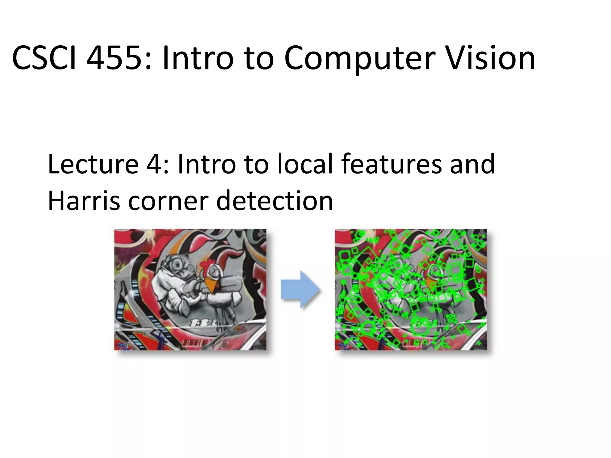
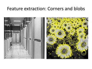
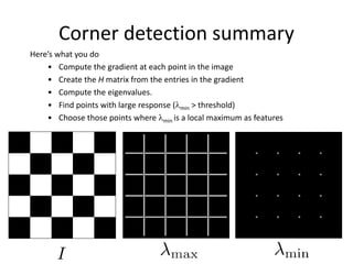
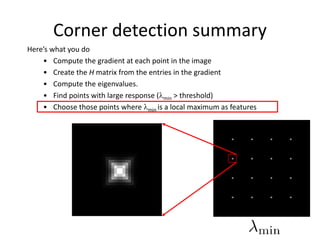
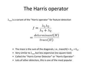
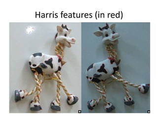
Harris corner detection is used to extract local features from images. It works by (1) computing the gradient at each point, (2) constructing a second moment matrix from the gradient, and (3) using the eigenvalues of this matrix to score how "corner-like" each point is. Points with a large, local maximum score are detected as corners. The Harris operator, which is a variant using the trace of the matrix, is commonly used due to its efficiency. Corners provide distinctive local features that can be matched between images.