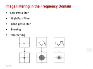
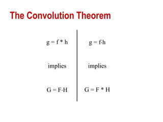
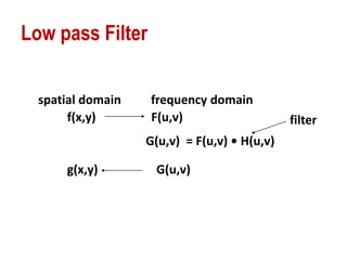
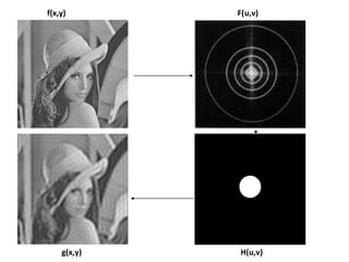
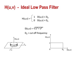
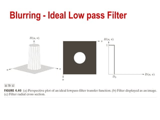
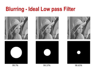
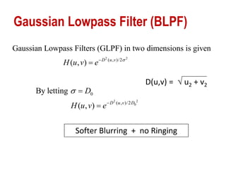
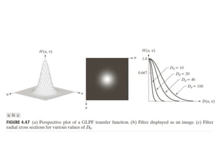
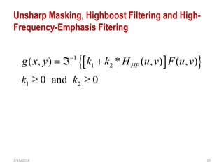
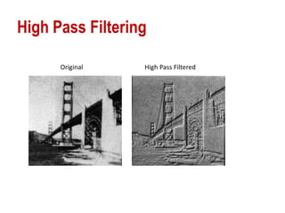
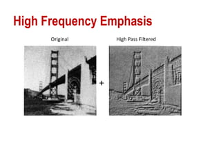
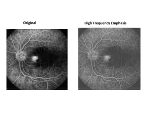
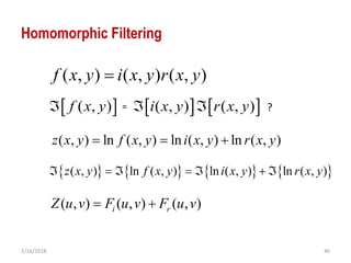
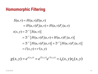
The document discusses various methods of digital image processing focusing on filtering in the frequency domain, including low pass, high pass, and band pass filters. It explains concepts such as the convolution theorem, various filter implementations (Butterworth, Gaussian), and techniques for image enhancement like unsharp masking and homomorphic filtering. Additionally, it covers selective filtering techniques like bandreject, bandpass, and notch filters, providing mathematical definitions and examples for each.

1. Digital Image
Processing

2. Image Filtering in the Frequency Domain
2/16/2018 2
• Low Pass Filter
• High Pass Filter
• Band pass Filter
• Blurring
• Sharpening

3. Frequency Bands
Percentage of image power enclosed in circles
(small to large) :
90, 95, 98, 99, 99.5, 99.9
Image Fourier Spectrum

4. Blurring - Ideal Low pass Filter
90%
95%
98%
99%
99.5% 99.9%

5. The Convolution Theorem
g = f * h g = fh
implies implies
G = FH G = F * H

6. Low pass Filter
f(x,y) F(u,v)
g(x,y) G(u,v)
G(u,v) = F(u,v) • H(u,v)
spatial domain frequency domain
filter

7. •
H(u,v)g(x,y)
f(x,y) F(u,v)
•

8. H(u,v) - Ideal Low Pass Filter
u
v
H(u,v)
0 D0
1
D(u,v)
H(u,v)
H(u,v) =
1 D(u,v)  D0
0 D(u,v) > D0
D(u,v) =  u2 + v2
D0 = cut off frequency

9. Blurring - Ideal Low pass Filter

10. Blurring - Ideal Low pass Filter
99.37%99.7% 98.65%

11. 98.0%
99.4%99.0%
96.6% 99.6%
99.7%

12. ILPF Filtering Example

14. The Ringing Problem
G(u,v) = F(u,v) • H(u,v)
g(x,y) = f(x,y) * h(x,y)
Convolution Theorem
sinc(x)
h(x,y)H(u,v)
 D0  Ringing radius +  blur
IFFT

15. 0 50 100 150 200 250
0
50
100
150
200
250
Freq. domain
Spatial domain

16. The Spatial Representation of ILPF

17. Butterworth Lowpass Filter (BLPF)
 
0
2
0
Butterworth Lowpass Filters (BLPF) of order and
with cutoff frequency
1
( , )
1 ( , ) /
n
n
D
H u v
D u v D



18. Butterworth Lowpass Filter (BLPF)

20. The Spatial Representation of BLPF

21. Gaussian Lowpass Filter (BLPF)
D(u,v) =  u2 + v2
Softer Blurring + no Ringing
2 2
( , )/2
Gaussian Lowpass Filters (GLPF) in two dimensions is given
( , ) D u v
H u v e 

2 2
0
0
( , )/2
By letting
( , ) D u v D
D
H u v e





24. Examples of smoothing by GLPF

25. Examples of smoothing by GLPF

26. Examples of smoothing by GLPF

27. Image Sharpening - High Pass Filters
A highpass filter is obtained from a given
lowpass filter using
( , ) 1 ( , )HP LPH u v H u v 
0
0
A 2-D ideal highpass filter (IHPL) is defined as
0 if ( , )
( , )
1 if ( , )
D u v D
H u v
D u v D

 


28.  
2
0
A 2-D Butterworth highpass filter (BHPL) is defined as
1
( , )
1 / ( , )
n
H u v
D D u v


2 2
0( , )/2
A 2-D Gaussian highpass filter (GHPL) is defined as
( , ) 1 D u v D
H u v e
 

30. The Spatial Representation of Highpass
Filters

31. Filtering Results by IHPF

32. Filtering Results by BHPF

33. Filtering Results by GHPF

34. 2/16/2018 34
Using Highpass Filtering and Threshold for Image
Enhancement
BHPF
(order 4 with a cutoff
frequency 50)

35. 2/16/2018 35
The Laplacian in the Frequency Domain
 2 1
The Laplacian image
( , ) ( , ) ( , )f x y H u v F u v
  
2 2 2
( , ) 4 ( )H u v u v  
2 2 2
2 2
( , ) 4 ( / 2) ( / 2) )
4 ( , )
H u v u P v Q
D u v


      
 
2
Enhancement is obtained
( , ) ( , ) ( , ) -1g x y f x y c f x y c   

36. 2/16/2018 36
The Laplacian in the Frequency Domain
 
  
 
1
1
1 2 2
The enhanced image
( , ) ( , ) ( , ) ( , )
1 ( , ) ( , )
1 4 ( , ) ( , )
g x y F u v H u v F u v
H u v F u v
D u v F u v



  
  
    

37. 2/16/2018 37
The Laplacian in the Frequency Domain

38. 2/16/2018 38
Unsharp Masking, Highboost Filtering and High-
Frequency-Emphasis Fitering
Unsharp masking and highboost filtering
( , ) ( , ) * ( , )maskg x y f x y k g x y 
( , ) ( , ) ( , )mask LPg x y f x y f x y 
 1
( , ) ( , ) ( , )LP LPf x y H u v F u v
 
  
  
1
1
( , ) 1 * 1 ( , ) ( , )
1 * ( , ) ( , )
LP
HP
g x y k H u v F u v
k H u v F u v


     
  

39. 2/16/2018 39
Unsharp Masking, Highboost Filtering and High-
Frequency-Emphasis Fitering
  1
1 2
1 2
( , ) * ( , ) ( , )
0 and 0
HPg x y k k H u v F u v
k k

  
 

40. High Pass Filtering
Original High Pass Filtered

41. High Frequency Emphasis
Original High Pass Filtered
+

42. Original High Frequency Emphasis

43. Original High Frequency Emphasis

44. 2/16/2018 45
Gaussian Filter
D0=40
High-Frequency-Emphasis Filtering
Gaussian Filter
K1=0.5, k2=0.75

45. 2/16/2018 46
Homomorphic Filtering
     ( , ) ( , ) ( , )f x y i x y r x y   
( , ) ( , ) ( , )f x y i x y r x y
( , ) ln ( , ) ln ( , ) ln ( , )z x y f x y i x y r x y  
= ?
       ( , ) ln ( , ) ln ( , ) ln ( , )z x y f x y i x y r x y      
( , ) ( , ) ( , )i rZ u v F u v F u v 

46. 2/16/2018 47
Homomorphic Filtering
 
 
   
1
1
1 1
( , ) ( , )
( , ) ( , ) ( , ) ( , )
( , ) ( , ) ( , ) ( , )
'( , ) '( , )
i r
i r
s x y S u v
H u v F u v H u v F u v
H u v F u v H u v F u v
i x y r x y


 
 
  
   
 
( , ) ( , ) ( , )
( , ) ( , ) ( , ) ( , )i r
S u v H u v Z u v
H u v F u v H u v F u v

 
( , ) '( , ) '( , )
0 0( , ) ( , ) ( , )s x y i x y r x y
g x y e e e i x y r x y  

47. 2/16/2018 48
Homomorphic Filtering
The illumination component of an image generally is
characterized by slow spatial variations, while the reflectance
component tends to vary abruptly
These characteristics lead to associating the low frequencies of
the Fourier transform of the logarithm of an image with
illumination the high frequencies with reflectance.

48. 2/16/2018 49
Homomorphic Filtering
2 2
0( , )/
( , ) ( ) 1
c D u v D
H L LH u v e  
 
     
  
Attenuate the contribution
made by illumination and
amplify the contribution made
by reflectance
Attenuate the contribution
made by illumination and
amplify the contribution made
by reflectance

49. 2/16/2018 50
Homomorphic Filtering
0
0.25
2
1
80
L
H
c
D







50. 2/16/2018 51
Homomorphic Filtering

51. 2/16/2018 52
Selective Filtering
Non-Selective Filters:
operate over the entire frequency rectangle
Selective Filters
operate over some part, not entire frequency rectangle
• bandreject or bandpass: process specific bands
• notch filters: process small regions of the frequency rectangle

52. 2/16/2018 53
Selective Filtering:
Bandreject and Bandpass Filters
( , ) 1 ( , )BP BRH u v H u v 

53. 2/16/2018 54
Selective Filtering:
Bandreject and Bandpass Filters

54. 2/16/2018 55
Selective Filtering:
Notch Filters
Zero-phase-shift filters must be symmetric about the origin.
A notch with center at (u0, v0) must have a corresponding notch
at location (-u0,-v0).
Notch reject filters are constructed as products of highpass filters
whose centers have been translated to the centers of the
notches.
1
-
( , ) ( , ) ( , )
where ( , ) and ( , ) are highpass filters whose centers are
at ( , ) and (- ,- ), respectively.
Q
NR k k
k
k k
k k k k
H u v H u v H u v
H u v H u v
u v u v


 

55. 2/16/2018 56
Selective Filtering:
Notch Filters
1
-
( , ) ( , ) ( , )
where ( , ) and ( , ) are highpass filters whose centers are
at ( , ) and (- ,- ), respectively.
Q
NR k k
k
k k
k k k k
H u v H u v H u v
H u v H u v
u v u v


 
1/22 2
1/22 2
( , ) ( / 2 ) ( / 2 )
( , ) ( / 2 ) ( / 2 )
k k k
k k k
D u v u M u v N v
D u v u M u v N v
       
       
   
3
2 2
1 0 0
A Butterworth notch reject filter of order n
1 1
( , )
1 / ( , ) 1 / ( , )
NR n n
k k k k k
H u v
D D u v D D u v 
   
    
       


56. 2/16/2018 57
Examples:
Notch Filters
(1)
0
A Butterworth notch
reject filter D =3
and n=4 for all
notch pairs

57. 2/16/2018 58
Examples:
Notch Filters (2)

58. 2/16/2018 59