Course: Machine Vision
Feature Detection
Session 06
D5627 – I Gede Putra Kusuma Negara, B.Eng., PhD
Outline
• Edge Detection
• Canny Edge Detector
• Interest Point and Corner
• Harris Corner Detector
Edge Detection
Detection Of Discontinuities
• There are three basic types of grey level discontinuities that
we tend to look for in digital images:
– Points
– Lines
– Edges
• We typically find discontinuities using masks and
correlation
Point Detection
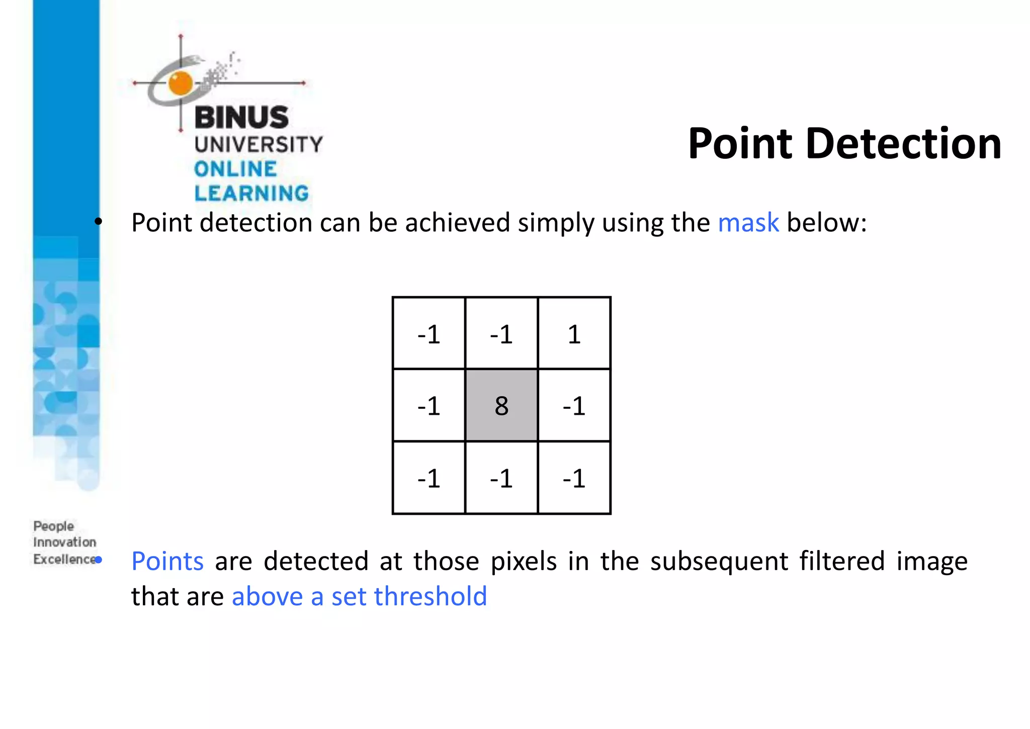
• Point detection can be achieved simply using the mask below:
• Points are detected at those pixels in the subsequent filtered image
that are above a set threshold
-1 -1 1
-1 8 -1
-1 -1 -1
Point Detection
X-ray image of a
turbine blade
Result of point
detection
Result of
thresholding
Line Detection
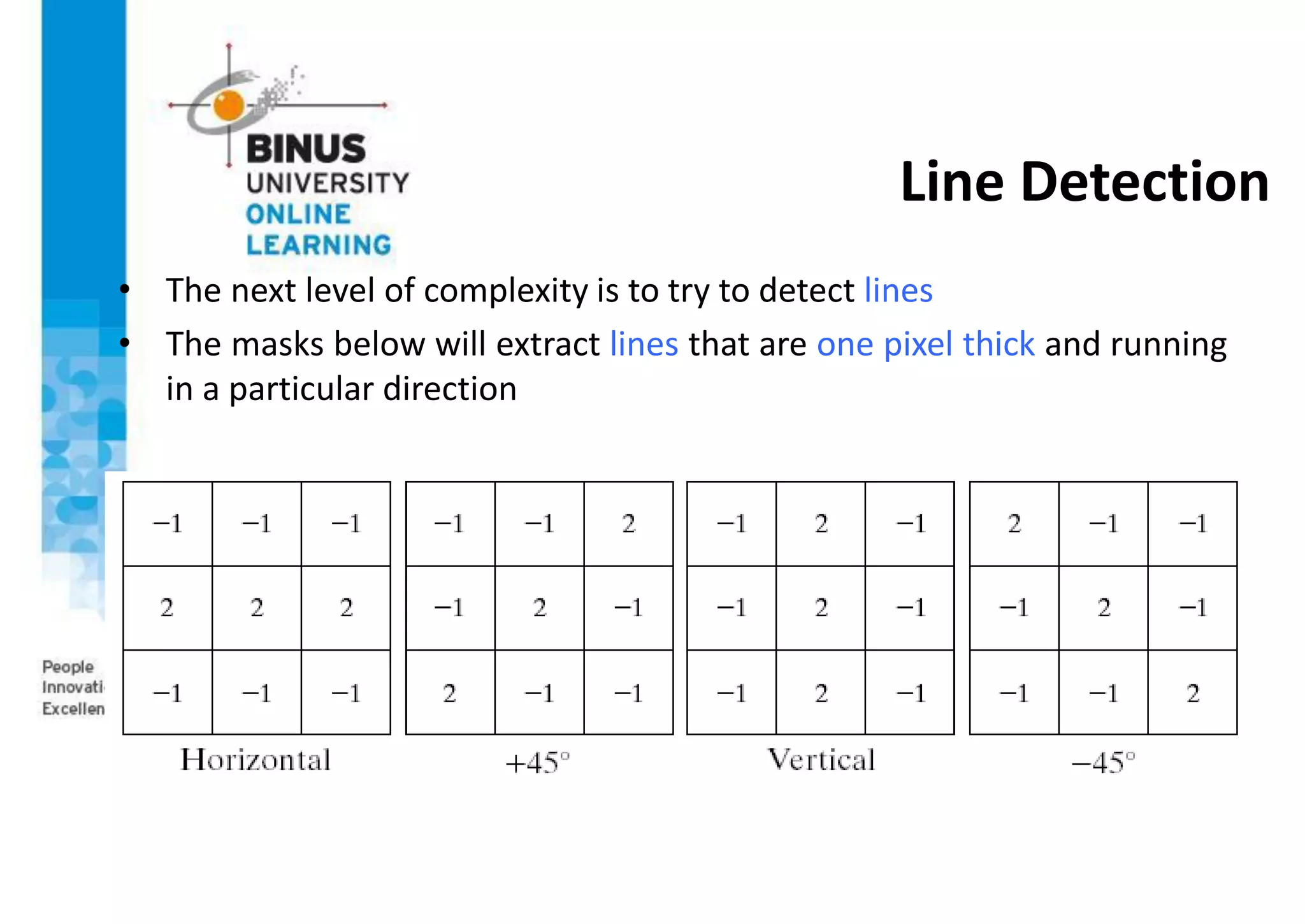
• The next level of complexity is to try to detect lines
• The masks below will extract lines that are one pixel thick and running
in a particular direction
Line Detection
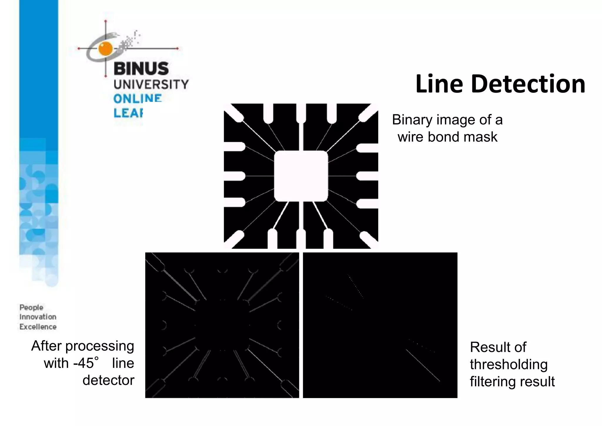
Binary image of a
wire bond mask
After processing
with -45° line
detector
Result of
thresholding
filtering result
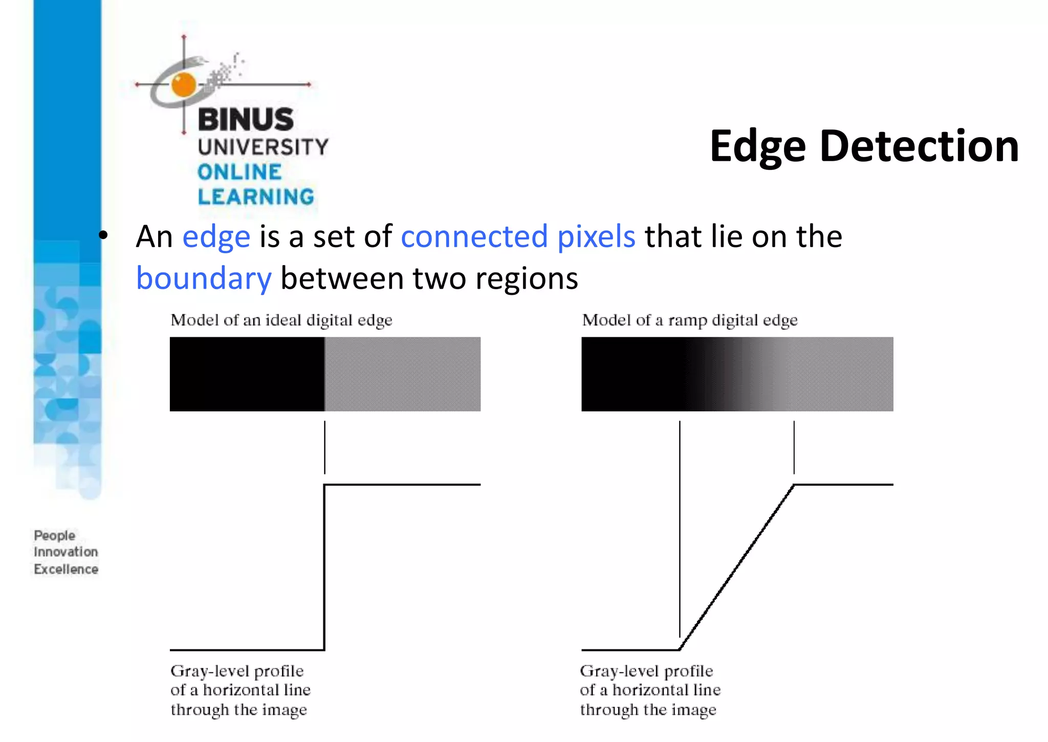
Edge Detection
• An edge is a set of connected pixels that lie on the
boundary between two regions
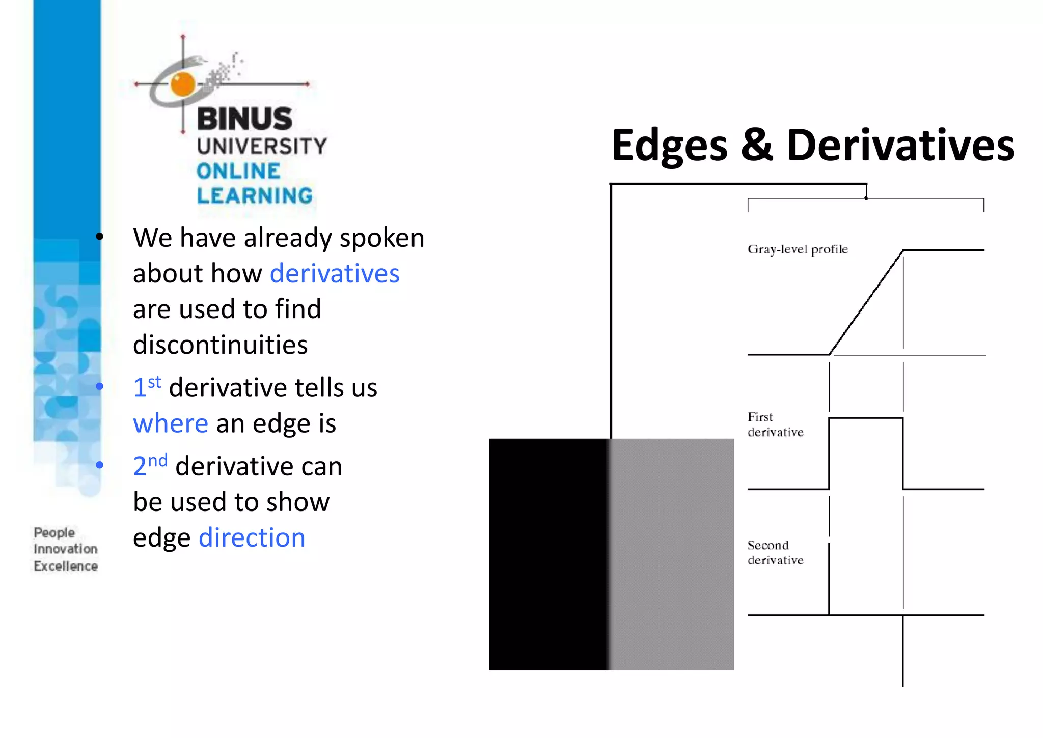
Edges & Derivatives
• We have already spoken
about how derivatives
are used to find
discontinuities
• 1st derivative tells us
where an edge is
• 2nd derivative can
be used to show
edge direction
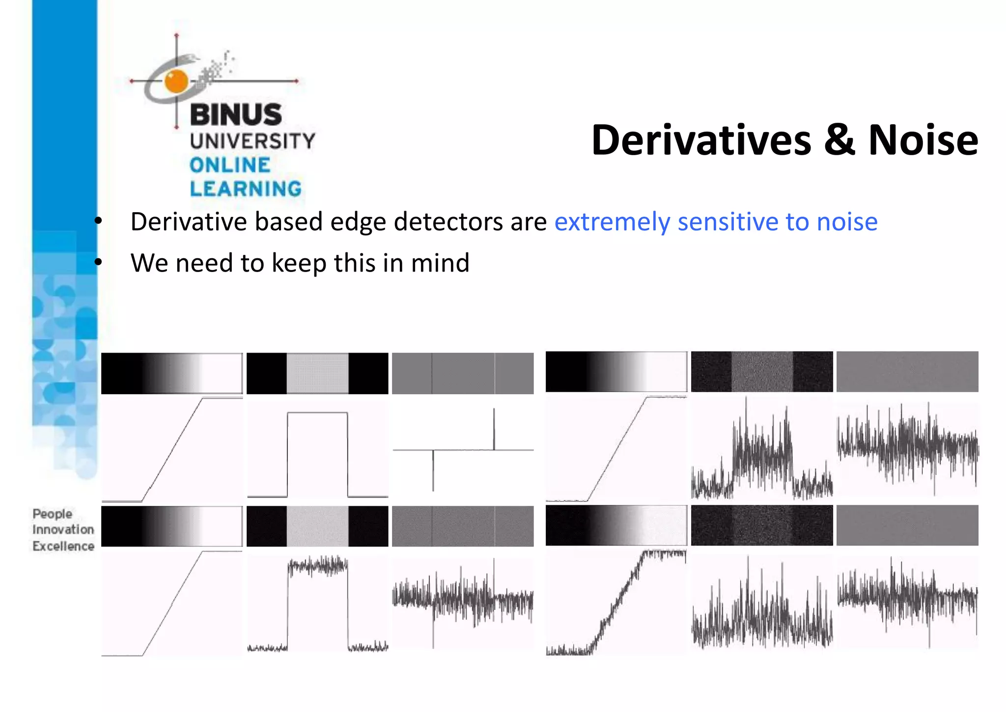
Derivatives & Noise
• Derivative based edge detectors are extremely sensitive to noise
• We need to keep this in mind
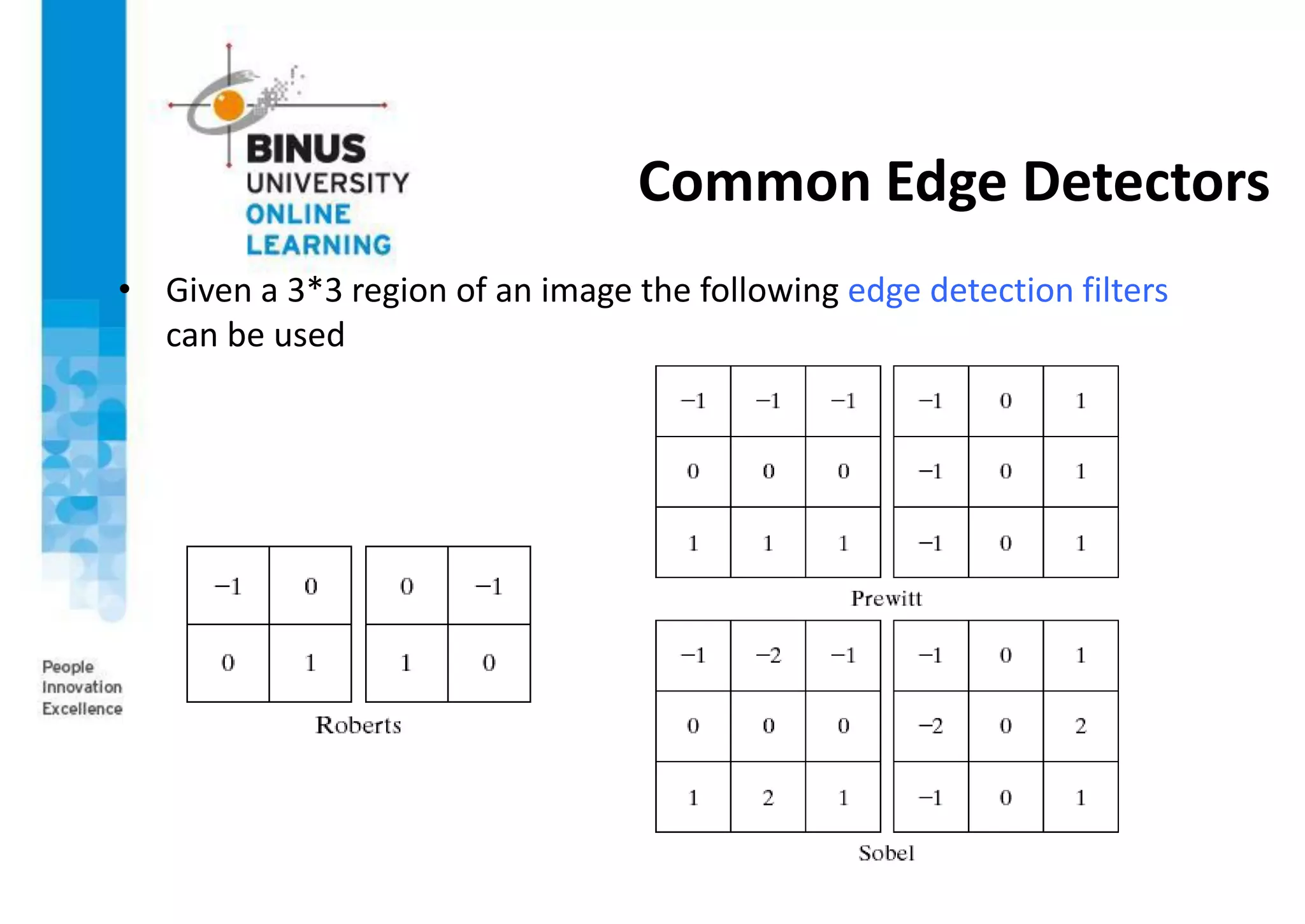
Common Edge Detectors
• Given a 3*3 region of an image the following edge detection filters
can be used
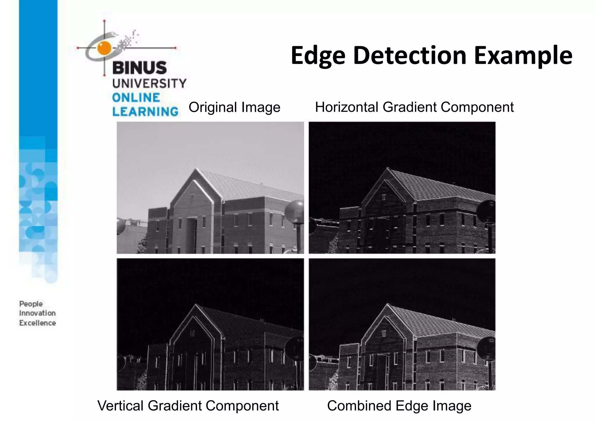
Edge Detection Example
Original Image Horizontal Gradient Component
Vertical Gradient Component Combined Edge Image
Edge Detection Problems
• Often, problems arise in edge detection in that there are is too much
detail
• For example, the brickwork in the previous example
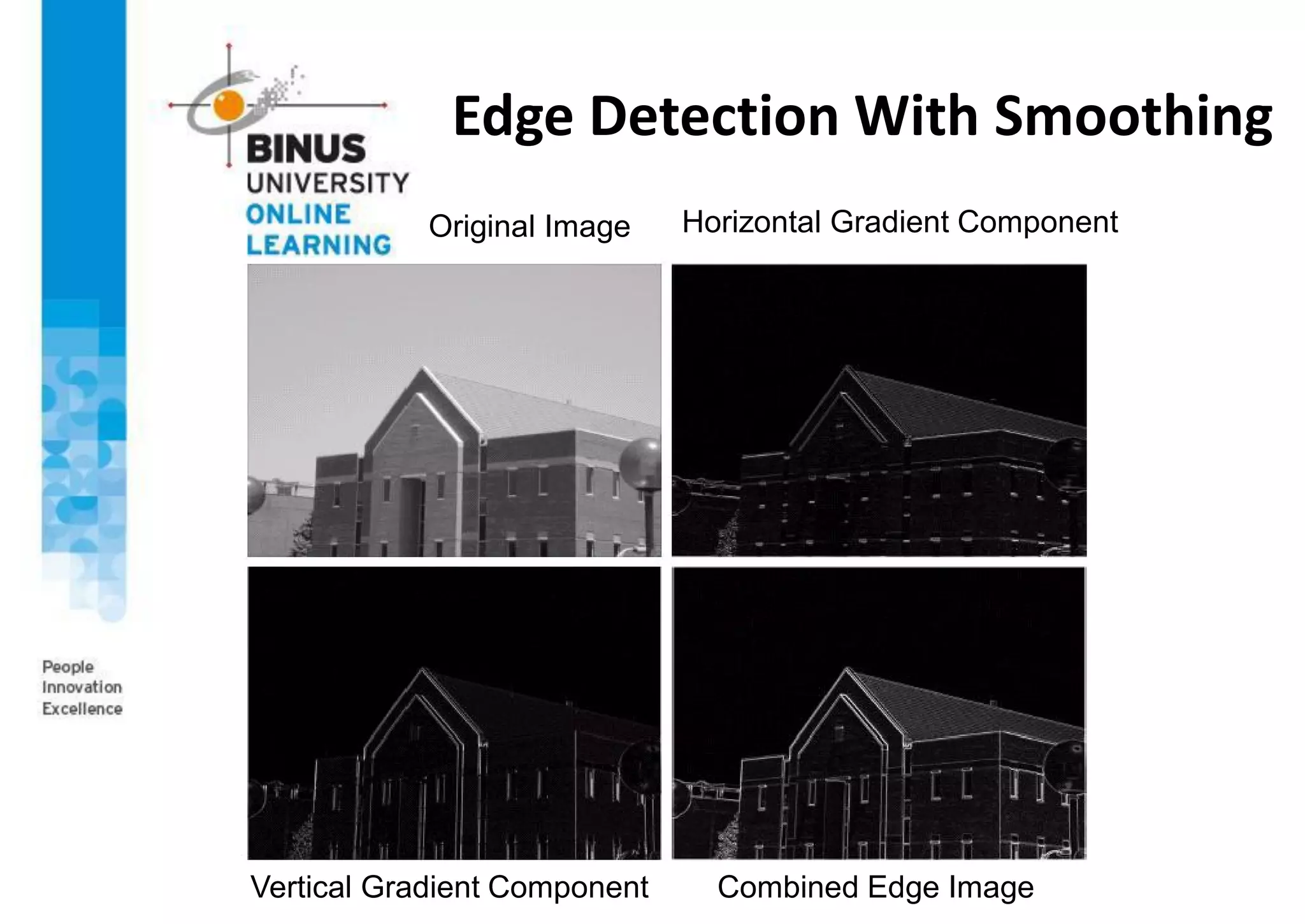
• One way to overcome this is to smooth images prior to edge
detection
Edge Detection With Smoothing
Original Image Horizontal Gradient Component
Vertical Gradient Component Combined Edge Image
Designing “Optimal”
Edge Detector
Criteria for an “optimal” edge detector:
• Good detection: the optimal detector must minimize the probability
of false positives (detecting spurious edges caused by noise), as well
as that of false negatives (missing real edges)
• Good localization: the edges detected must be as close as possible to
the true edges
• Single response: the detector must return one point only for each true
edge point; that is, minimize the number of local maxima around the
true edge
Canny Edge Detector
• This is probably the most widely used edge detector in computer
vision
• Theoretical model: step-edges corrupted by additive Gaussian noise
• Canny has shown that the first derivative of the Gaussian closely
approximates the operator that optimizes the product of signal- to-
noise ratio and localization
Canny Edge Detector
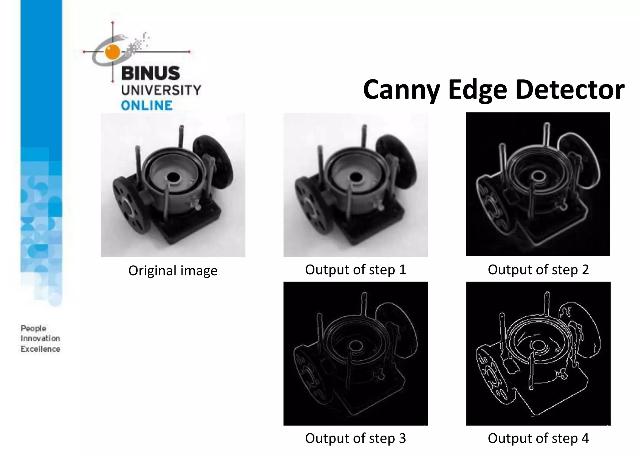
1. Filter image with derivative of Gaussian
2. Find magnitude and orientation of gradient
3. Non-maximum suppression:
Thin multi-pixel wide “ridges” down to single pixel width
4. Linking and thresholding (hysteresis):
Define two thresholds: low and high
Use the high threshold to start edge curves and the low threshold to
continue them
Canny Edge Detector
Original image Output of step 1 Output of step 2
Output of step 3 Output of step 4
Interest Points
Interest Points
• Feature detection and matching are an essential component of many
computer vision applications
• For example, we are going to align following images so they can be
seamlessly stitched into composite mosaic
Interest Points
• What kinds of features should you detect and then match in order to
establish such an alignment?
• The first kind of feature that we may notice are specific locations in
the images, such as mountain peaks, or interestingly shaped patches
of snow
• These kinds of localized feature are often called keypoint features or
interest points and are often described by the appearance of patches
of pixels surrounding the point location
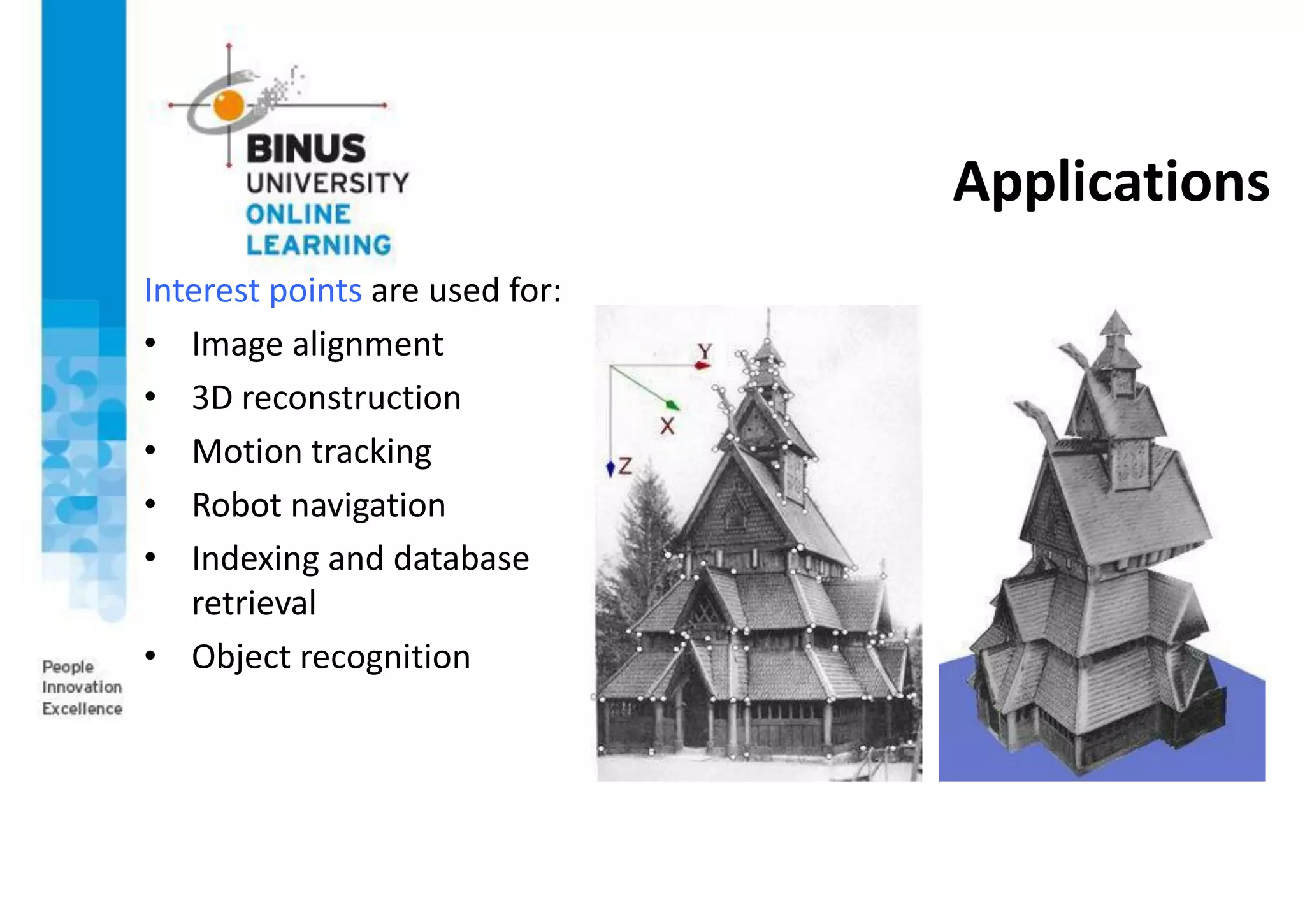
Applications
Interest points are used for:
• Image alignment
• 3D reconstruction
• Motion tracking
• Robot navigation
• Indexing and database
retrieval
• Object recognition
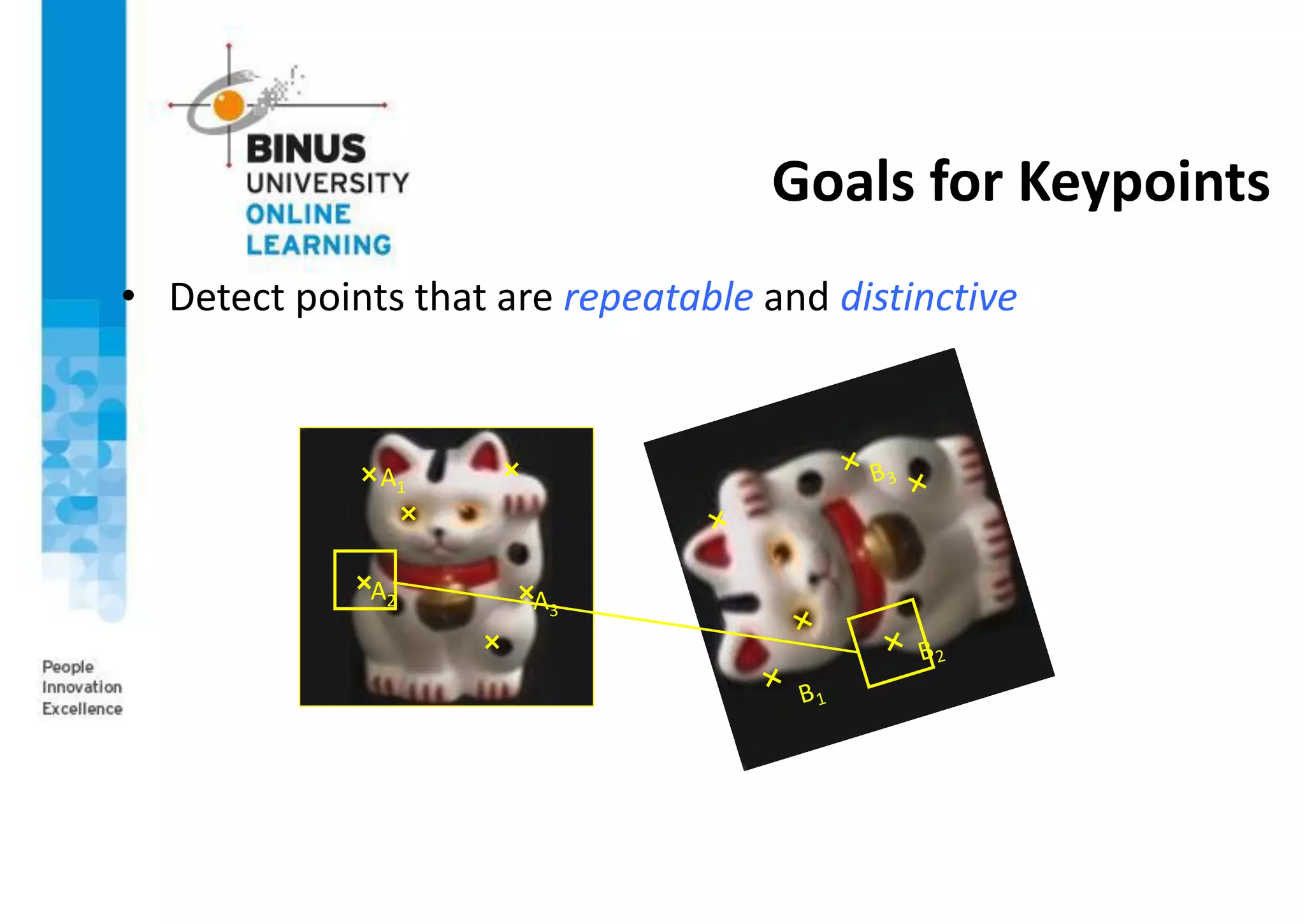
Goals for Keypoints
• Detect points that are repeatable and distinctive
A1
A2 A3
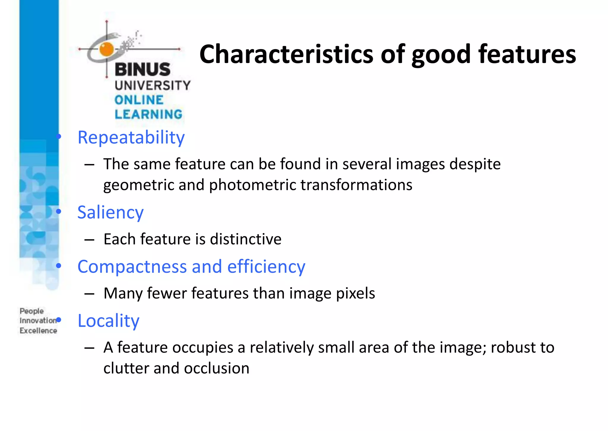
Characteristics of good features
• Repeatability
– The same feature can be found in several images despite
geometric and photometric transformations
• Saliency
– Each feature is distinctive
• Compactness and efficiency
– Many fewer features than image pixels
• Locality
– A feature occupies a relatively small area of the image; robust to
clutter and occlusion
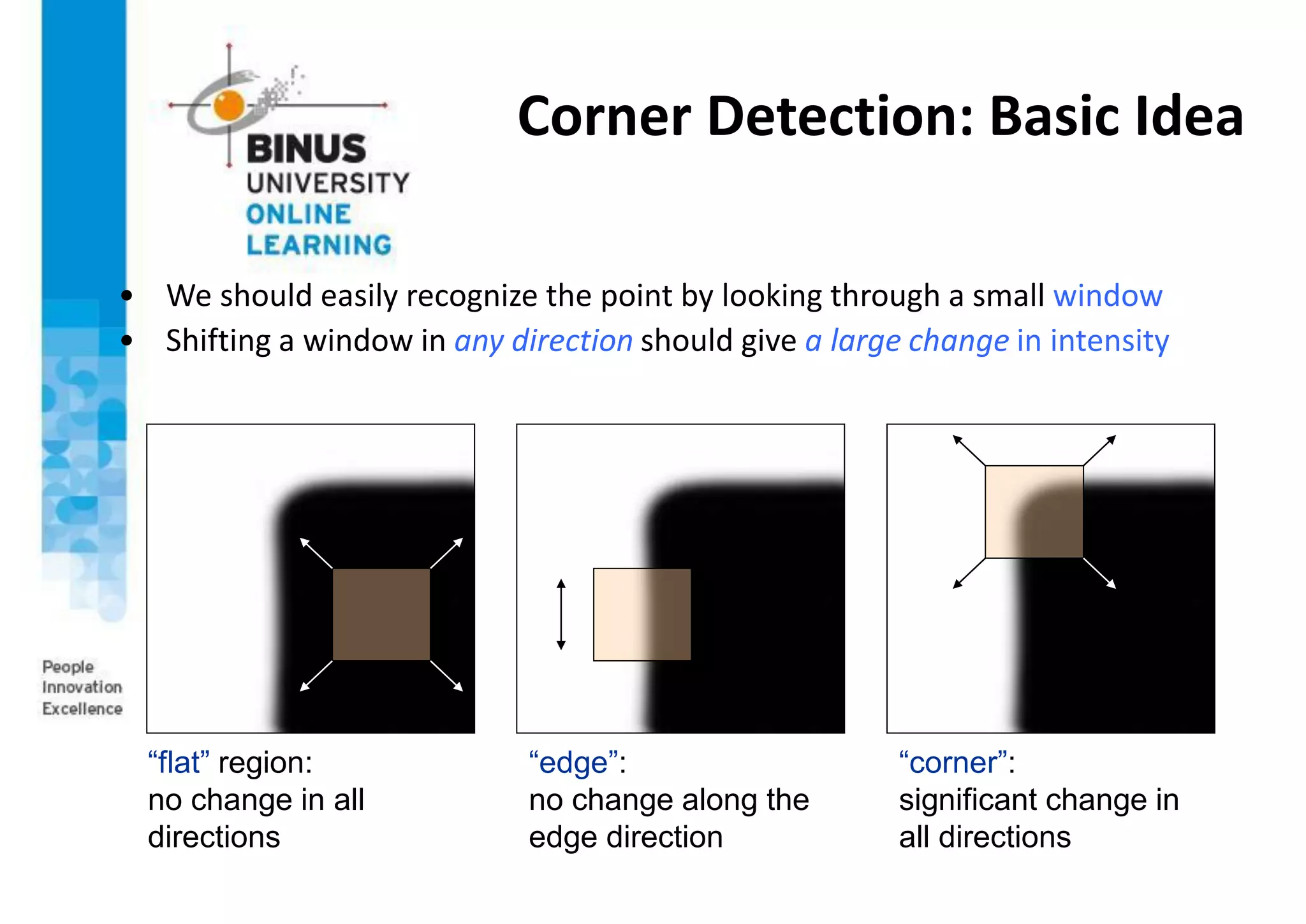
Corner Detection: Basic Idea
• We should easily recognize the point by looking through a small window
• Shifting a window in any direction should give a large change in intensity
“edge”:
no change along the
edge direction
“corner”:
significant change in
all directions
“flat” region:
no change in all
directions
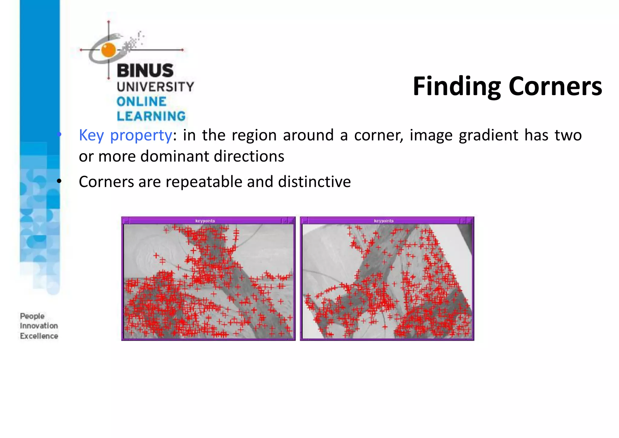
Finding Corners
• Key property: in the region around a corner, image gradient has two
or more dominant directions
• Corners are repeatable and distinctive
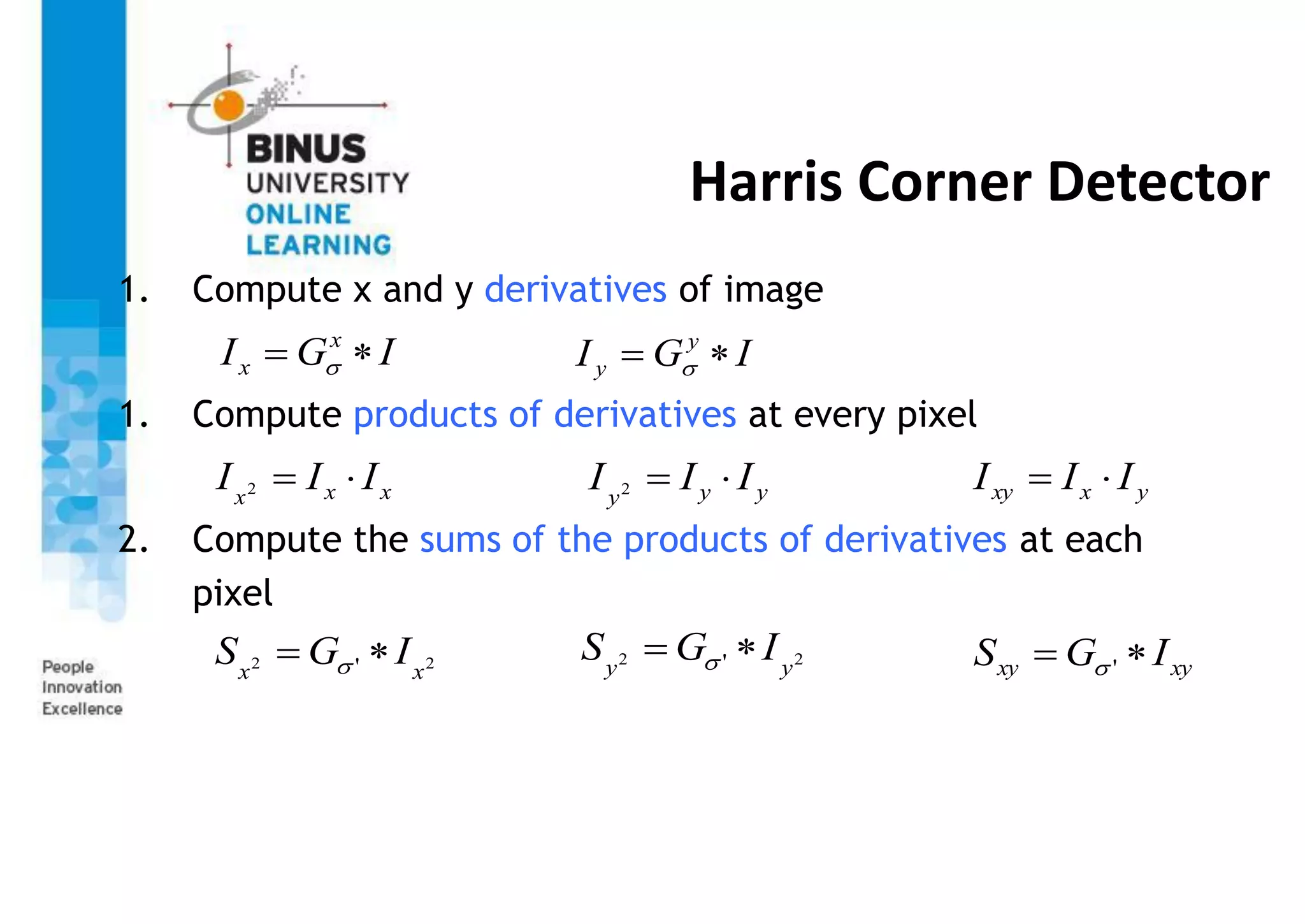
Harris Corner Detector
1. Compute x and y derivatives of image
1. Compute products of derivatives at every pixel
2. Compute the sums of the products of derivatives at each
pixel
I
G
I x
x 
  I
G
I y
y 
 
x
x
x
I
I
I 

2 y
y
y
I
I
I 

2 y
x
xy I
I
I 

2
2 ' x
x
I
G
S 
  2
2 ' y
y
I
G
S 
  xy
xy I
G
S 
 '

Harris Corner Detector
4. Define the matrix at each pixel
5. Compute the response of the detector at each pixel
6. Threshold on value of R; compute non-max suppression
25-Jun-21 Image Processing and Multimedia Retrieval 29









)
,
(
)
,
(
)
,
(
)
,
(
)
,
(
2
2
y
x
S
y
x
S
y
x
S
y
x
S
y
x
M
y
xy
xy
x
 2
trace
det M
k
M
R 

= g(Ix
2
)g(Iy
2
)-[g(IxIy )]2
-a[g(Ix
2
)+g(Iy
2
)]2
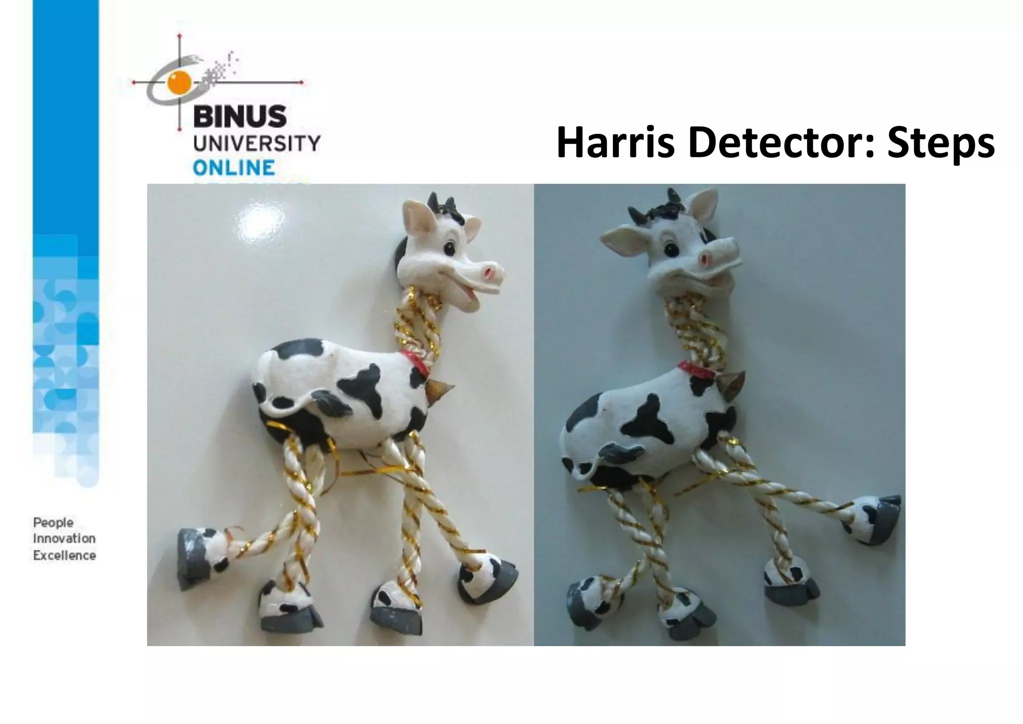
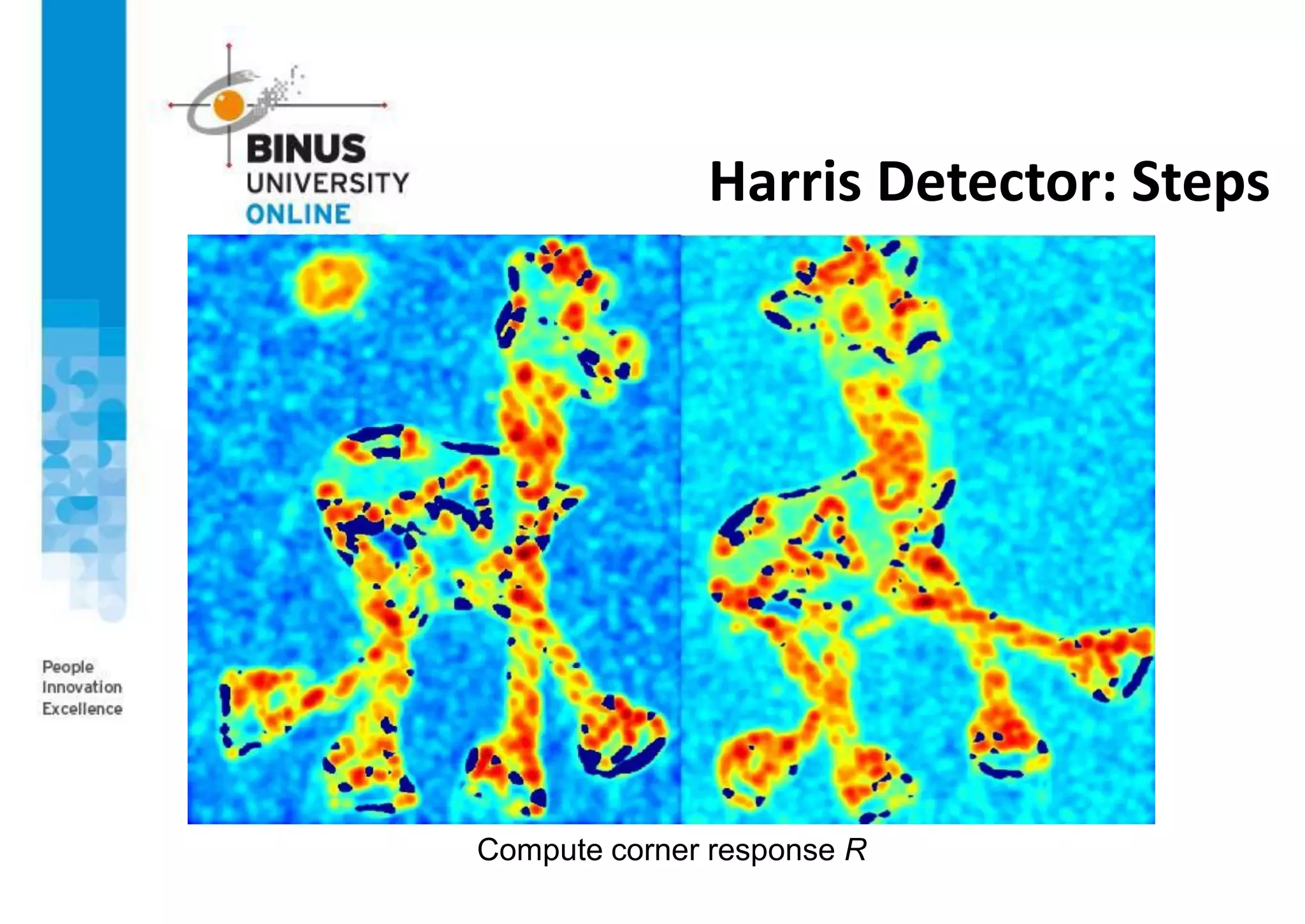
Harris Detector: Steps
Compute corner response R
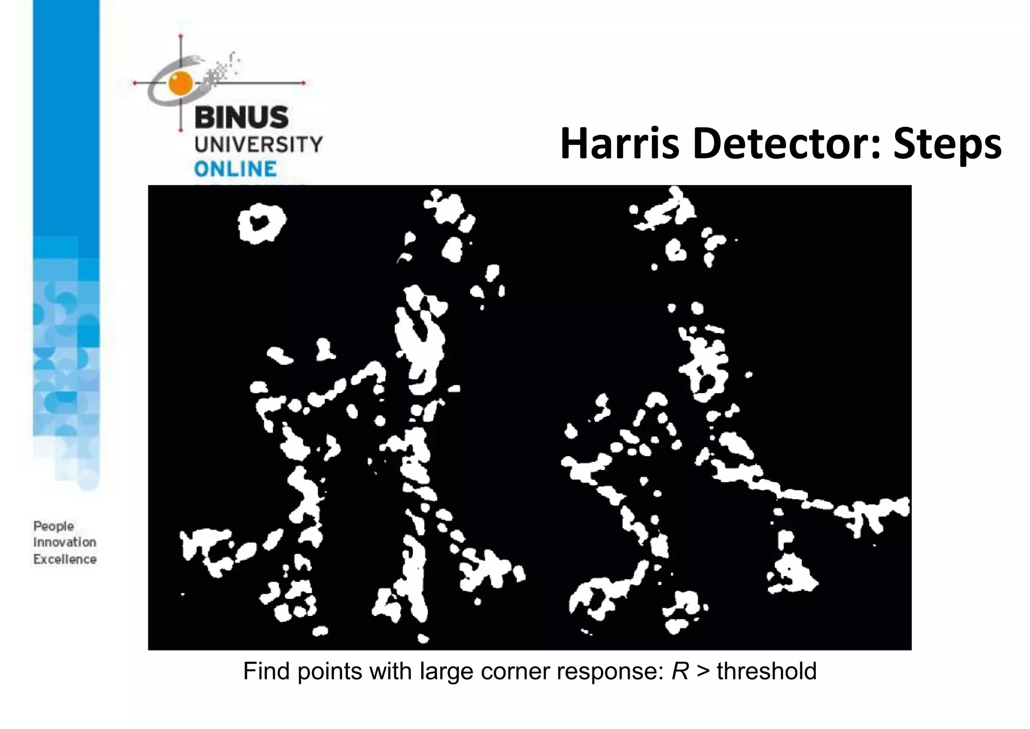
Harris Detector: Steps
Find points with large corner response: R > threshold
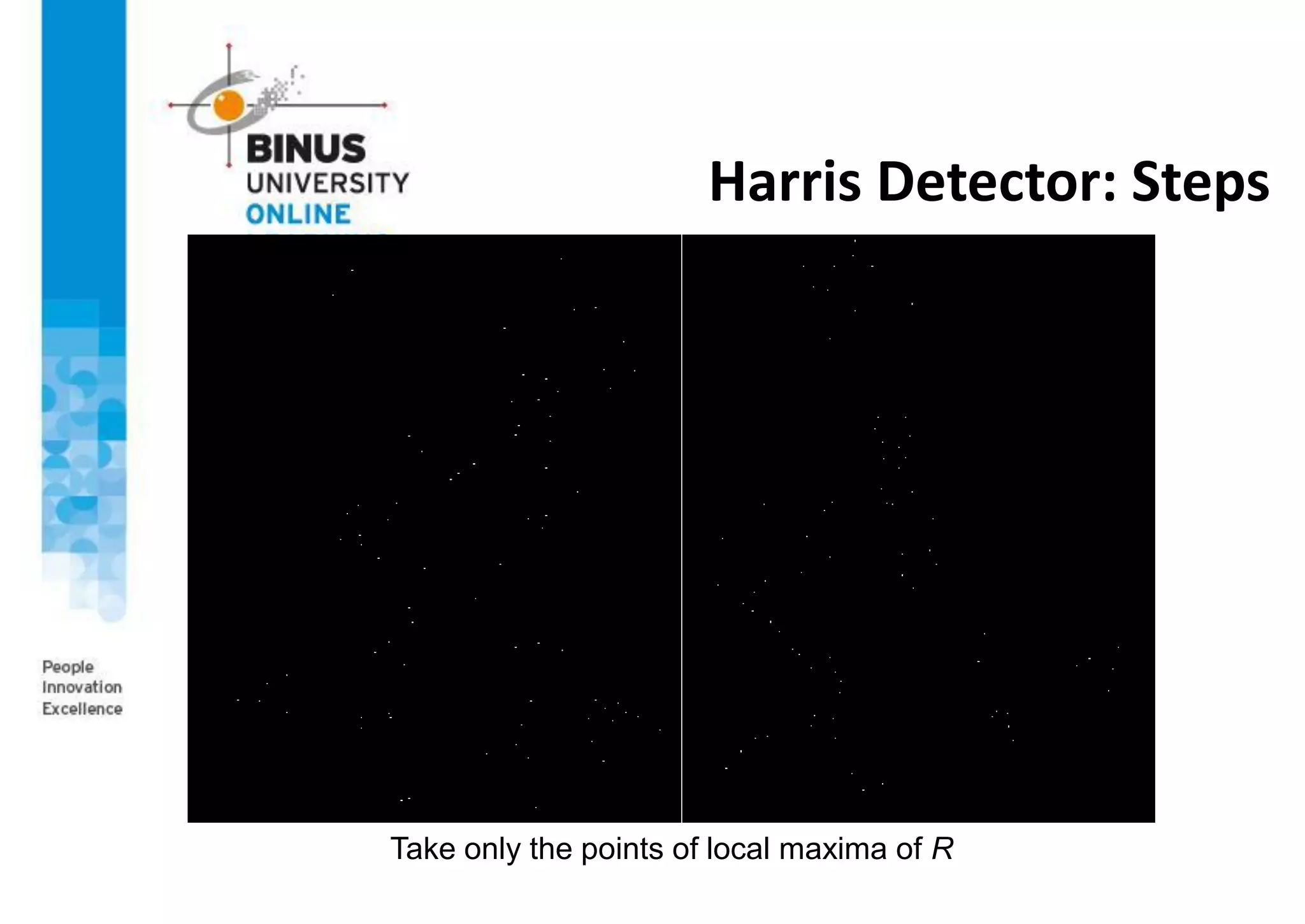
Harris Detector: Steps
Take only the points of local maxima of R
Harris Detector: Steps
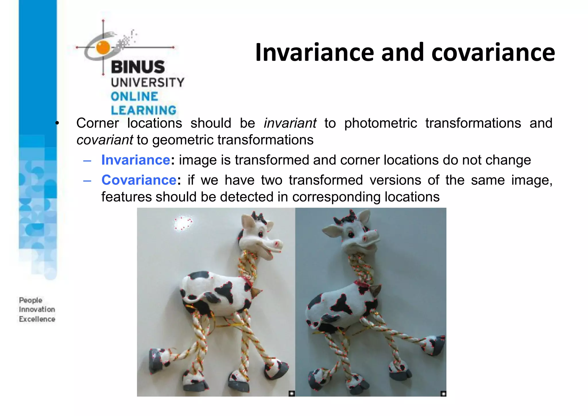
Invariance and covariance
• Corner locations should be invariant to photometric transformations and
covariant to geometric transformations
– Invariance: image is transformed and corner locations do not change
– Covariance: if we have two transformed versions of the same image,
features should be detected in corresponding locations
Acknowledgment
Some of slides in this PowerPoint presentation are adaptation from
various slides, many thanks to:
1. Dr. Brian Mac Namee, School of Computing at the Dublin Institute
of Technology (http://www.comp.dit.ie/bmacnamee/gaip.htm)
2. James Hays, Computer Science Department, Brown University,
(http://cs.brown.edu/~hays/)
Thank You

PPT s06-machine vision-s2

  • 1.
    Course: Machine Vision FeatureDetection Session 06 D5627 – I Gede Putra Kusuma Negara, B.Eng., PhD
  • 2.
    Outline • Edge Detection •Canny Edge Detector • Interest Point and Corner • Harris Corner Detector
  • 3.
  • 4.
    Detection Of Discontinuities •There are three basic types of grey level discontinuities that we tend to look for in digital images: – Points – Lines – Edges • We typically find discontinuities using masks and correlation
  • 5.
    Point Detection • Pointdetection can be achieved simply using the mask below: • Points are detected at those pixels in the subsequent filtered image that are above a set threshold -1 -1 1 -1 8 -1 -1 -1 -1
  • 6.
    Point Detection X-ray imageof a turbine blade Result of point detection Result of thresholding
  • 7.
    Line Detection • Thenext level of complexity is to try to detect lines • The masks below will extract lines that are one pixel thick and running in a particular direction
  • 8.
    Line Detection Binary imageof a wire bond mask After processing with -45° line detector Result of thresholding filtering result
  • 9.
    Edge Detection • Anedge is a set of connected pixels that lie on the boundary between two regions
  • 10.
    Edges & Derivatives •We have already spoken about how derivatives are used to find discontinuities • 1st derivative tells us where an edge is • 2nd derivative can be used to show edge direction
  • 11.
    Derivatives & Noise •Derivative based edge detectors are extremely sensitive to noise • We need to keep this in mind
  • 12.
    Common Edge Detectors •Given a 3*3 region of an image the following edge detection filters can be used
  • 13.
    Edge Detection Example OriginalImage Horizontal Gradient Component Vertical Gradient Component Combined Edge Image
  • 14.
    Edge Detection Problems •Often, problems arise in edge detection in that there are is too much detail • For example, the brickwork in the previous example • One way to overcome this is to smooth images prior to edge detection
  • 15.
    Edge Detection WithSmoothing Original Image Horizontal Gradient Component Vertical Gradient Component Combined Edge Image
  • 16.
    Designing “Optimal” Edge Detector Criteriafor an “optimal” edge detector: • Good detection: the optimal detector must minimize the probability of false positives (detecting spurious edges caused by noise), as well as that of false negatives (missing real edges) • Good localization: the edges detected must be as close as possible to the true edges • Single response: the detector must return one point only for each true edge point; that is, minimize the number of local maxima around the true edge
  • 17.
    Canny Edge Detector •This is probably the most widely used edge detector in computer vision • Theoretical model: step-edges corrupted by additive Gaussian noise • Canny has shown that the first derivative of the Gaussian closely approximates the operator that optimizes the product of signal- to- noise ratio and localization
  • 18.
    Canny Edge Detector 1.Filter image with derivative of Gaussian 2. Find magnitude and orientation of gradient 3. Non-maximum suppression: Thin multi-pixel wide “ridges” down to single pixel width 4. Linking and thresholding (hysteresis): Define two thresholds: low and high Use the high threshold to start edge curves and the low threshold to continue them
  • 19.
    Canny Edge Detector Originalimage Output of step 1 Output of step 2 Output of step 3 Output of step 4
  • 20.
  • 21.
    Interest Points • Featuredetection and matching are an essential component of many computer vision applications • For example, we are going to align following images so they can be seamlessly stitched into composite mosaic
  • 22.
    Interest Points • Whatkinds of features should you detect and then match in order to establish such an alignment? • The first kind of feature that we may notice are specific locations in the images, such as mountain peaks, or interestingly shaped patches of snow • These kinds of localized feature are often called keypoint features or interest points and are often described by the appearance of patches of pixels surrounding the point location
  • 23.
    Applications Interest points areused for: • Image alignment • 3D reconstruction • Motion tracking • Robot navigation • Indexing and database retrieval • Object recognition
  • 24.
    Goals for Keypoints •Detect points that are repeatable and distinctive A1 A2 A3
  • 25.
    Characteristics of goodfeatures • Repeatability – The same feature can be found in several images despite geometric and photometric transformations • Saliency – Each feature is distinctive • Compactness and efficiency – Many fewer features than image pixels • Locality – A feature occupies a relatively small area of the image; robust to clutter and occlusion
  • 26.
    Corner Detection: BasicIdea • We should easily recognize the point by looking through a small window • Shifting a window in any direction should give a large change in intensity “edge”: no change along the edge direction “corner”: significant change in all directions “flat” region: no change in all directions
  • 27.
    Finding Corners • Keyproperty: in the region around a corner, image gradient has two or more dominant directions • Corners are repeatable and distinctive
  • 28.
    Harris Corner Detector 1.Compute x and y derivatives of image 1. Compute products of derivatives at every pixel 2. Compute the sums of the products of derivatives at each pixel I G I x x    I G I y y    x x x I I I   2 y y y I I I   2 y x xy I I I   2 2 ' x x I G S    2 2 ' y y I G S    xy xy I G S   ' 
  • 29.
    Harris Corner Detector 4.Define the matrix at each pixel 5. Compute the response of the detector at each pixel 6. Threshold on value of R; compute non-max suppression 25-Jun-21 Image Processing and Multimedia Retrieval 29          ) , ( ) , ( ) , ( ) , ( ) , ( 2 2 y x S y x S y x S y x S y x M y xy xy x  2 trace det M k M R   = g(Ix 2 )g(Iy 2 )-[g(IxIy )]2 -a[g(Ix 2 )+g(Iy 2 )]2
  • 30.
  • 31.
  • 32.
    Harris Detector: Steps Findpoints with large corner response: R > threshold
  • 33.
    Harris Detector: Steps Takeonly the points of local maxima of R
  • 34.
  • 35.
    Invariance and covariance •Corner locations should be invariant to photometric transformations and covariant to geometric transformations – Invariance: image is transformed and corner locations do not change – Covariance: if we have two transformed versions of the same image, features should be detected in corresponding locations
  • 36.
    Acknowledgment Some of slidesin this PowerPoint presentation are adaptation from various slides, many thanks to: 1. Dr. Brian Mac Namee, School of Computing at the Dublin Institute of Technology (http://www.comp.dit.ie/bmacnamee/gaip.htm) 2. James Hays, Computer Science Department, Brown University, (http://cs.brown.edu/~hays/)
  • 37.