Feature detection and
description
Can you match the scene
points?
o Detection
o Descriptio
n
o Matching
Feature
detection
“flat”
region: no
change in
all
directions
Slide adapted from Darya Frolova, Denis Simakov, Weizmann
“edge”: no
change
along the
edge
direction
“corner”:
significant
change in
all
directions
A local measure for uniquely identifying the
feature.

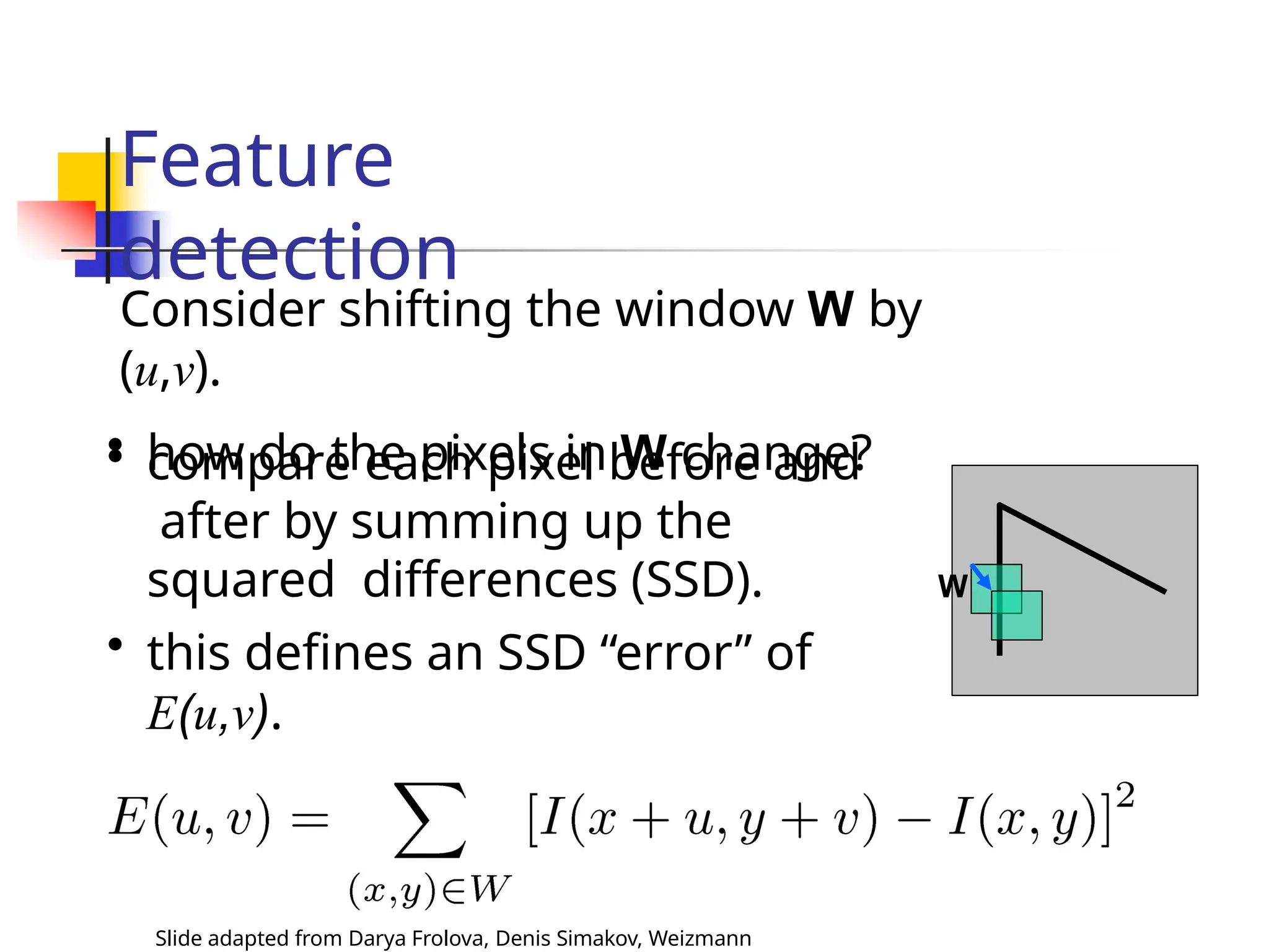
How does the measure change on shifting
windows at different points?
• compare each pixel before and
after by summing up the
squared differences (SSD).
• this defines an SSD “error” of
E(u,v).
Feature
detection
Consider shifting the window W by
(u,v).
• how do the pixels in W change?
W
Slide adapted from Darya Frolova, Denis Simakov, Weizmann
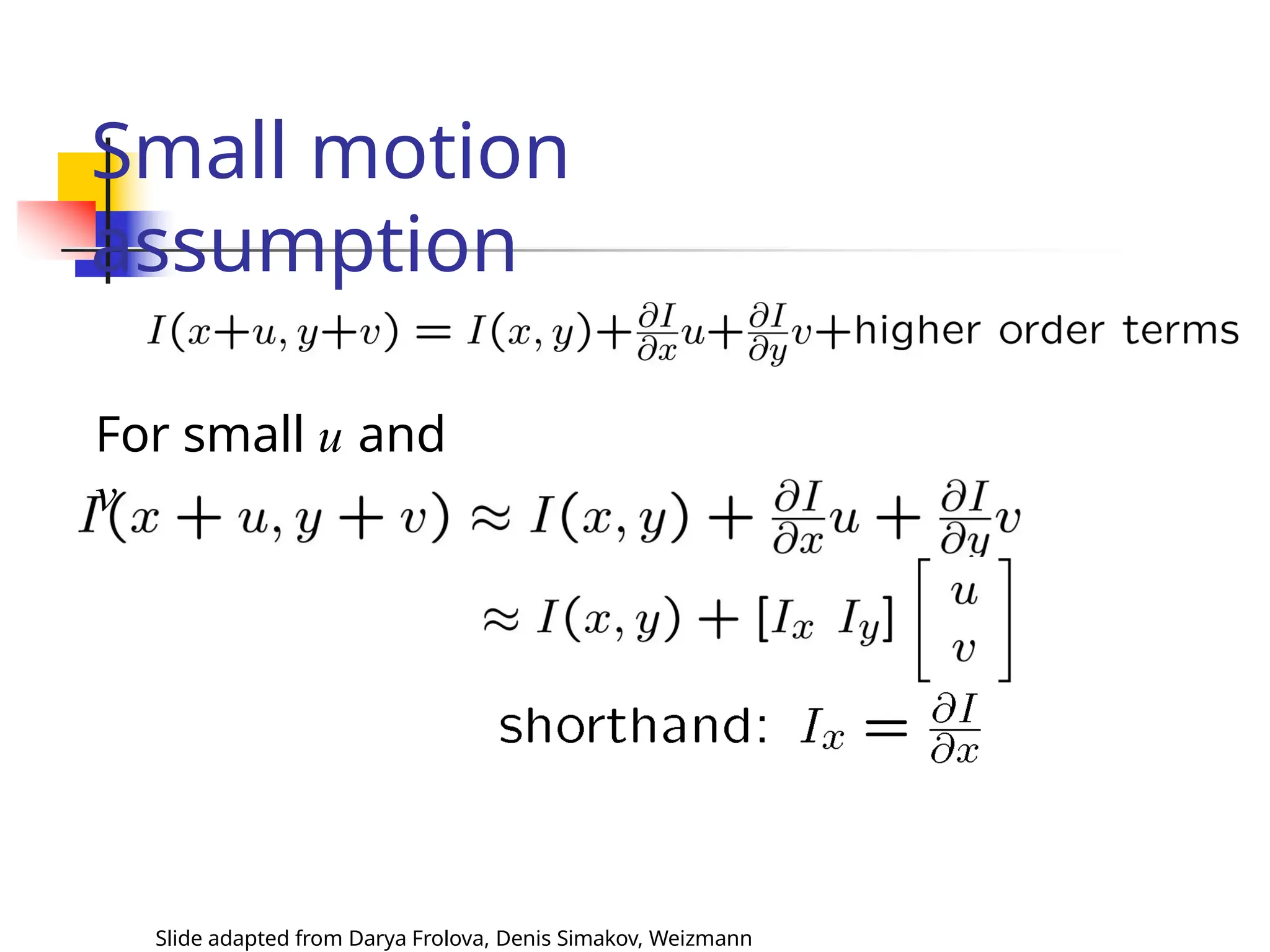
Small motion
assumption
For small u and
v
Slide adapted from Darya Frolova, Denis Simakov, Weizmann
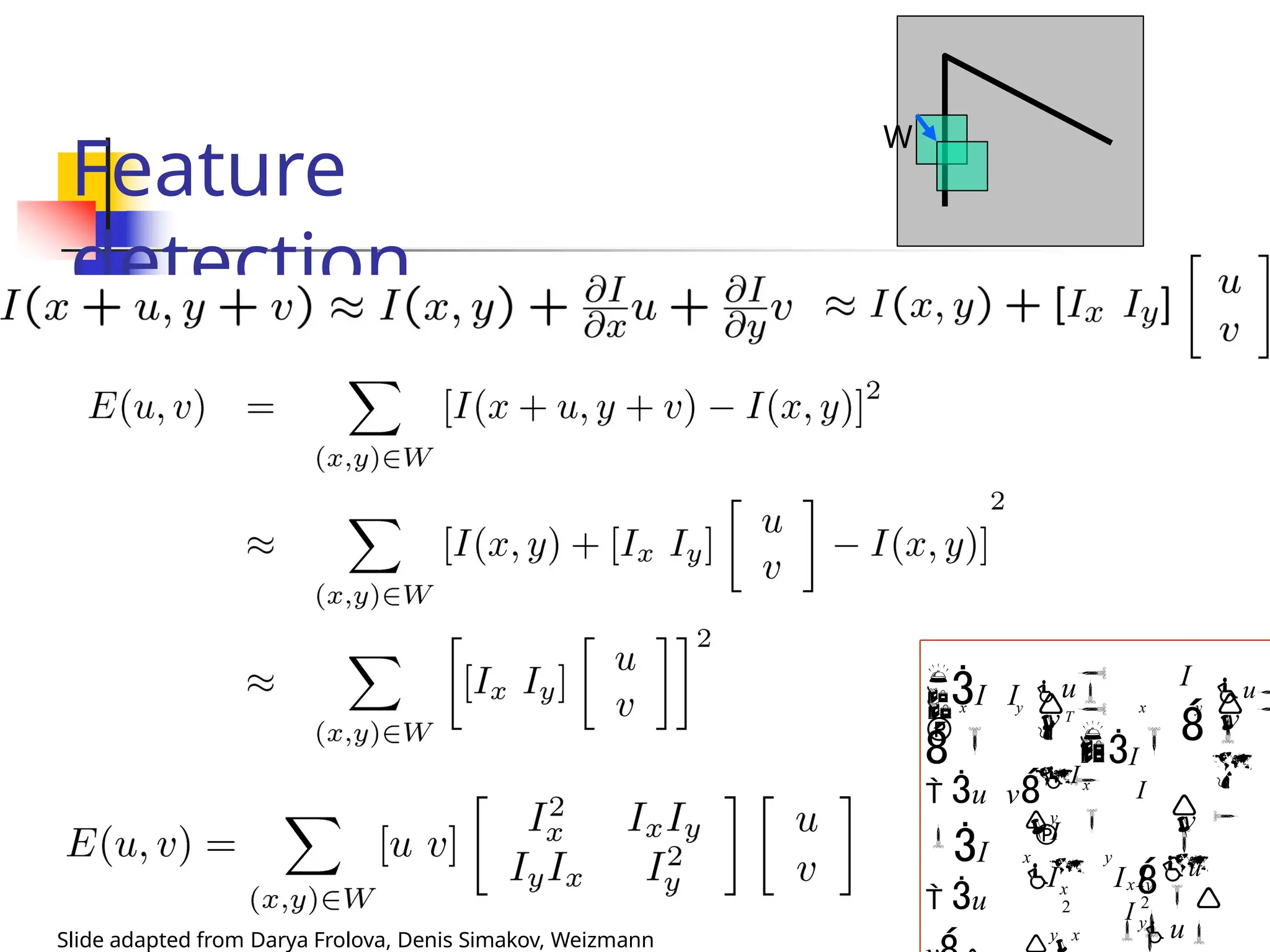
Feature
detection
W



















I I
u
I
 u
v
I
u

v
u


I


I
v
I I

y
y x
x
I 
x y
 u vI x

I
x y 

u

T

x y 

x y
I 2 

y

2
Slide adapted from Darya Frolova, Denis Simakov, Weizmann
Feature
detection
For the example above
• Suppose the center of the green
window moved to anywhere on the
blue unit circle.
• Directions for the largest and the
smallest E
values?
• Eigenvectors of H.
Slide adapted from Darya Frolova, Denis Simakov, Weizmann
Quick
eigenvalue/eigenvector
review
The eigenvectors of a matrix A are the vectors x that
satisfy:
The scalar  is the eigenvalue corresponding to x
 The eigenvalues are found by solving:
 For eigen vector solve the following:
Once you know , you find eigen vector [x y]T by solving
the
above Slide adapted from Darya Frolova, Denis Simakov, Weizmann
Feature
detection
Eigenvalues and eigenvectors of H
• Define shifts with the smallest
and largest change (E value)
• x+ = direction of largest increase
in E.
• + = amount of increase in
direction x+
x-
x+
Slide adapted from Darya Frolova, Denis Simakov, Weizmann
Feature scoring
function
Slide adapted from Darya Frolova, Denis Simakov, Weizmann
E(u,v) to be large for small shifts in all
directions
• the minimum of E(u,v) should be
large, over all unit vectors [u v].
• this minimum is given by the
smaller eigenvalue (-) of H
Feature
detection
Slide adapted from Darya Frolova, Denis Simakov, Weizmann
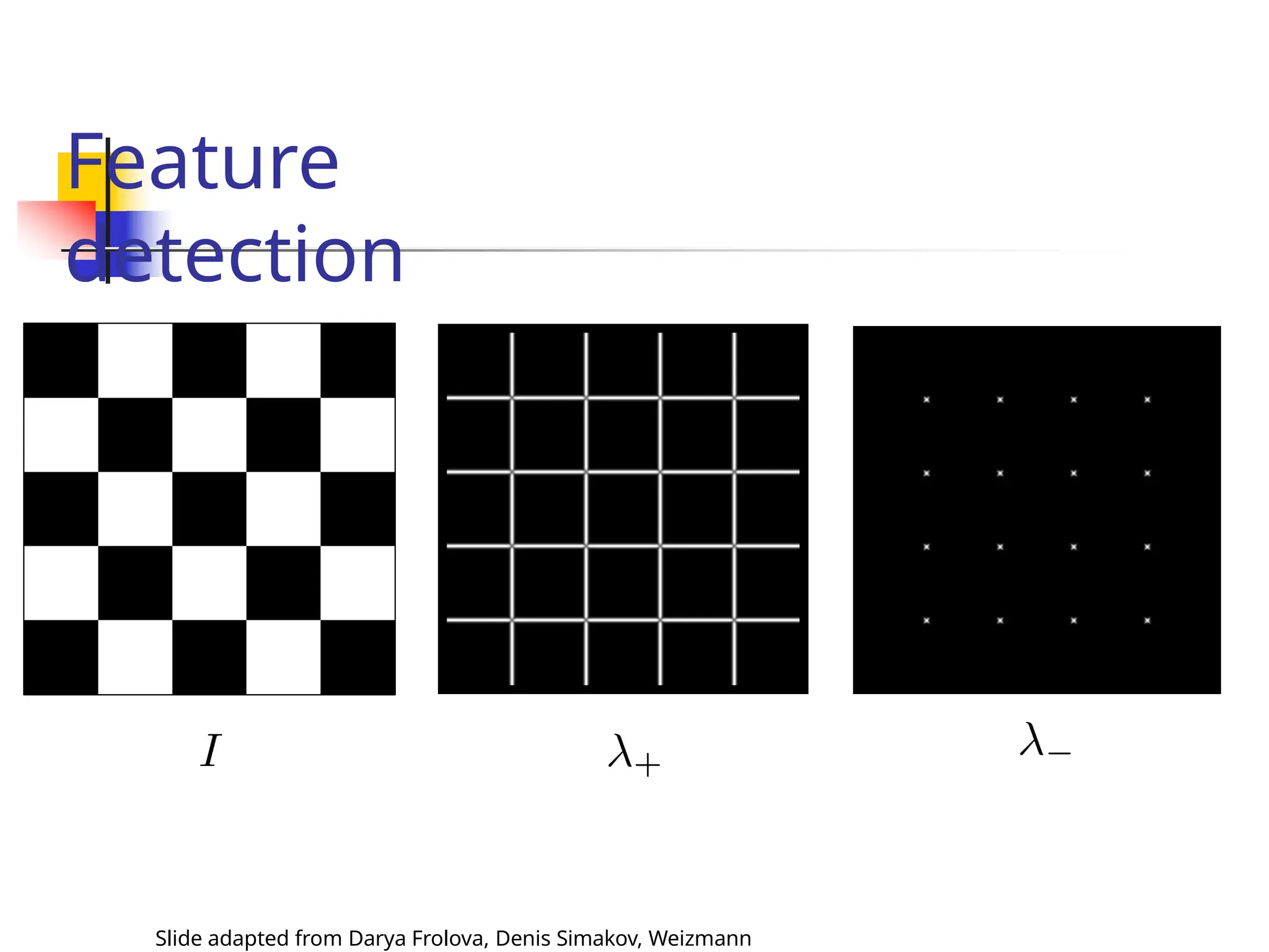
Feature detection:
Algorithm
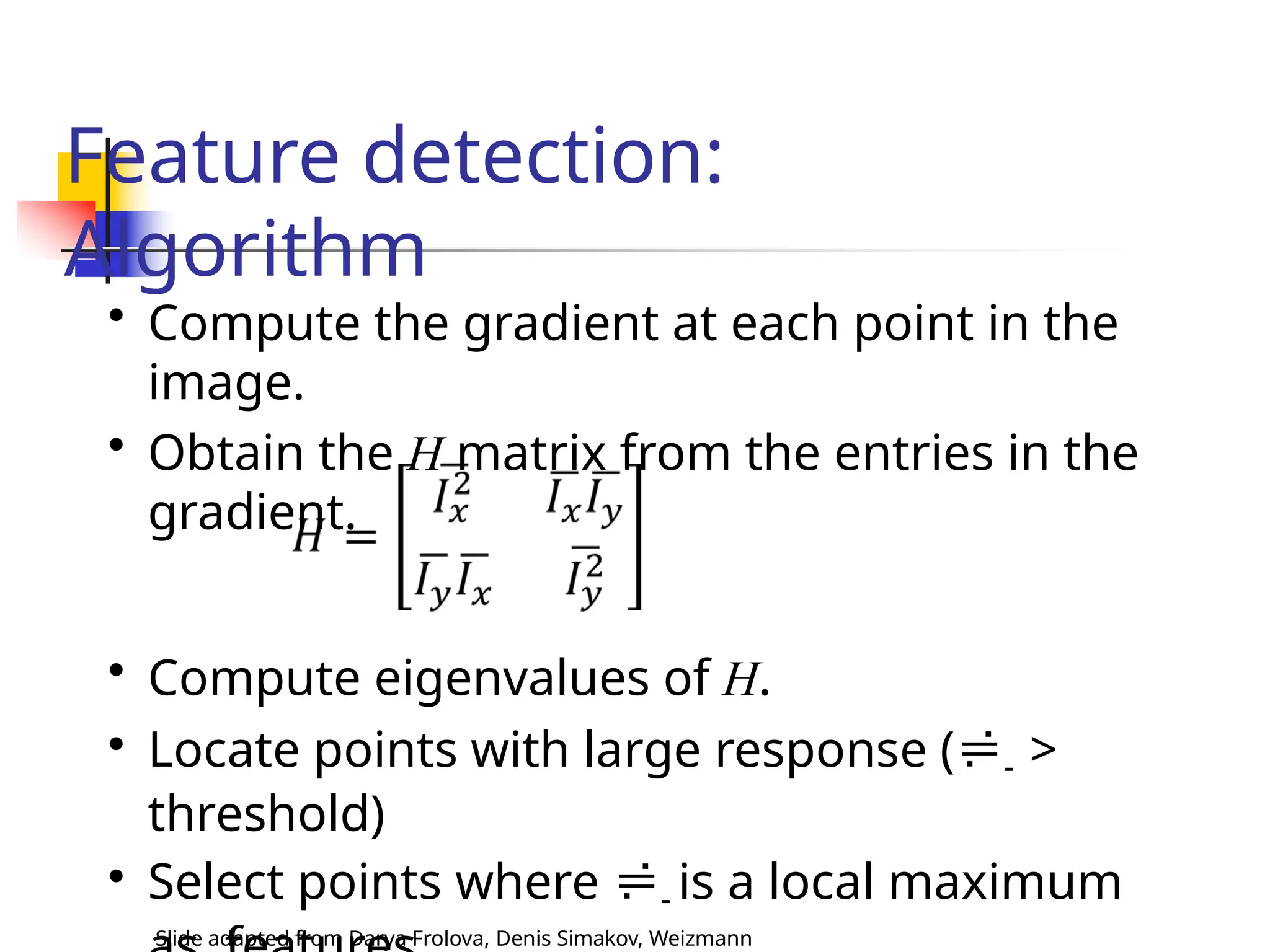
• Compute the gradient at each point in the
image.
• Obtain the H matrix from the entries in the
gradient.
• Compute eigenvalues of H.
• Locate points with large response (- >
threshold)
• Select points where - is a local maximum
Slide adapted from Darya Frolova, Denis Simakov, Weizmann
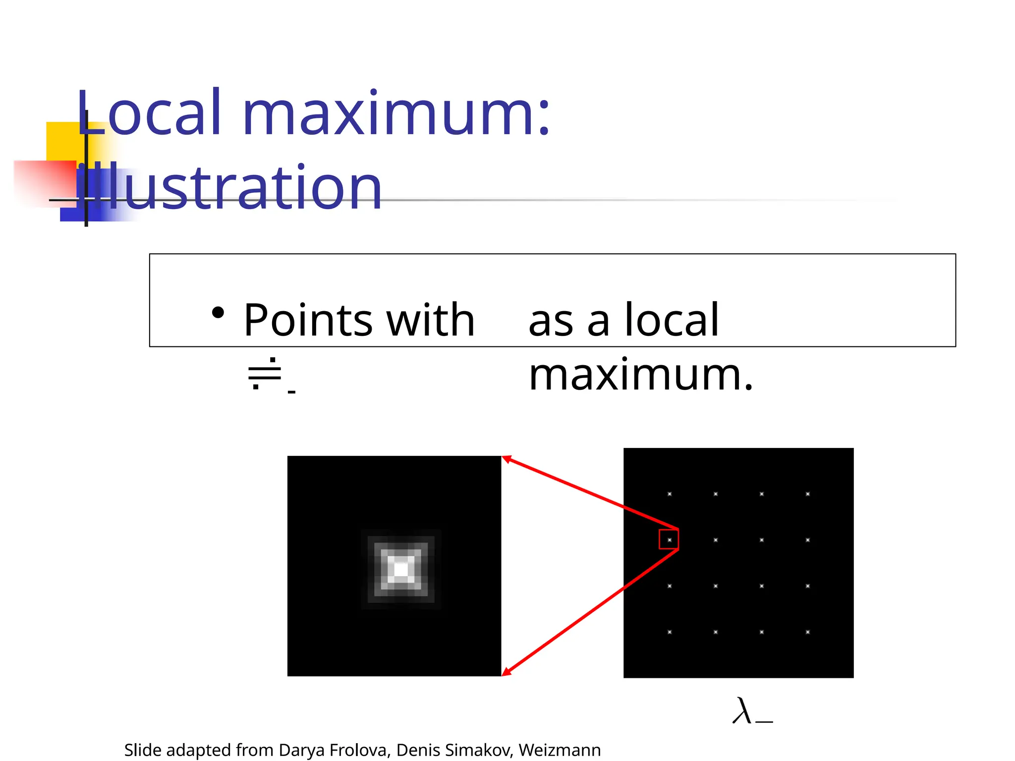
Local maximum:
illustration
• Points with
-
Slide adapted from Darya Frolova, Denis Simakov, Weizmann
as a local
maximum.
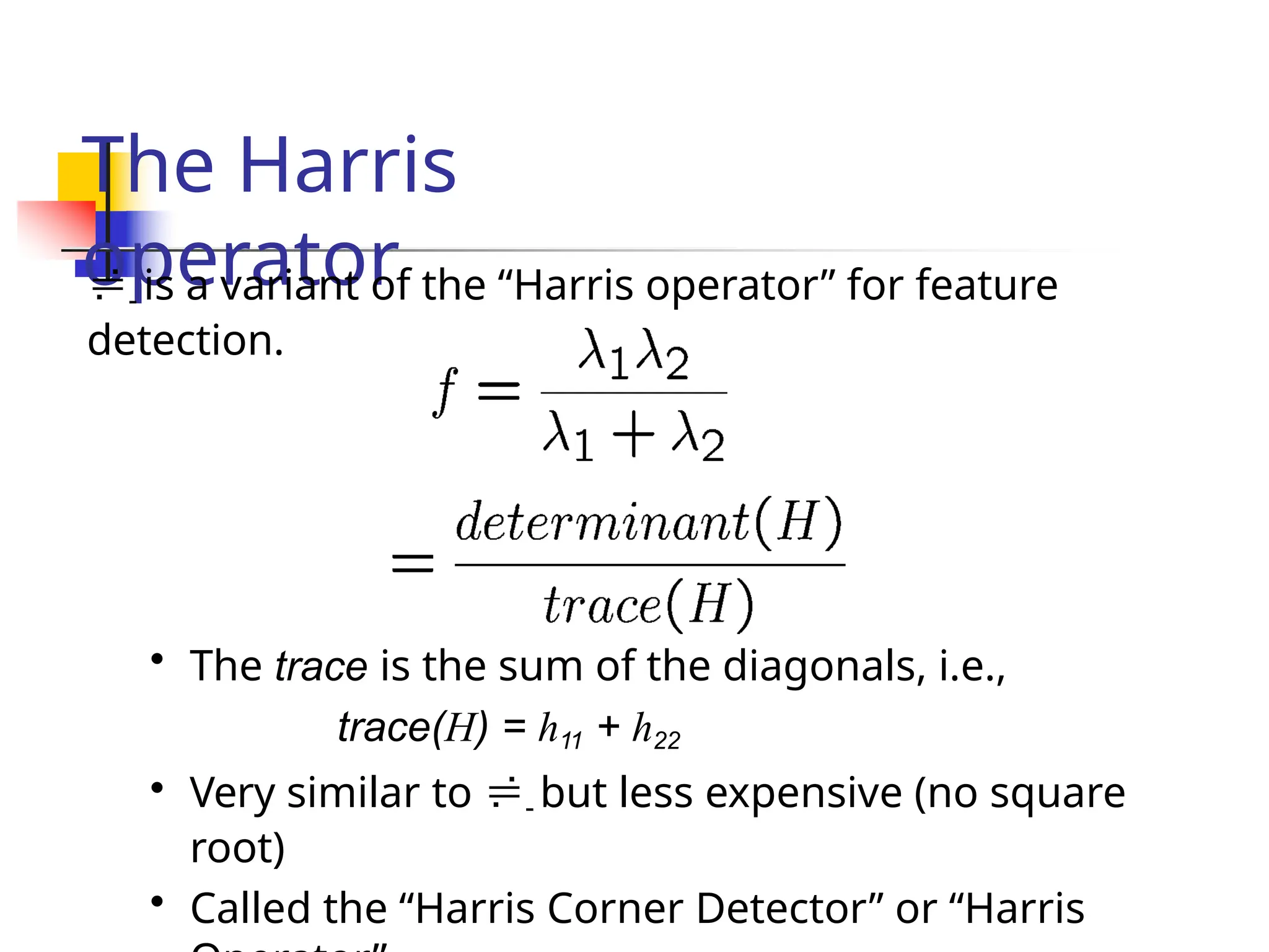
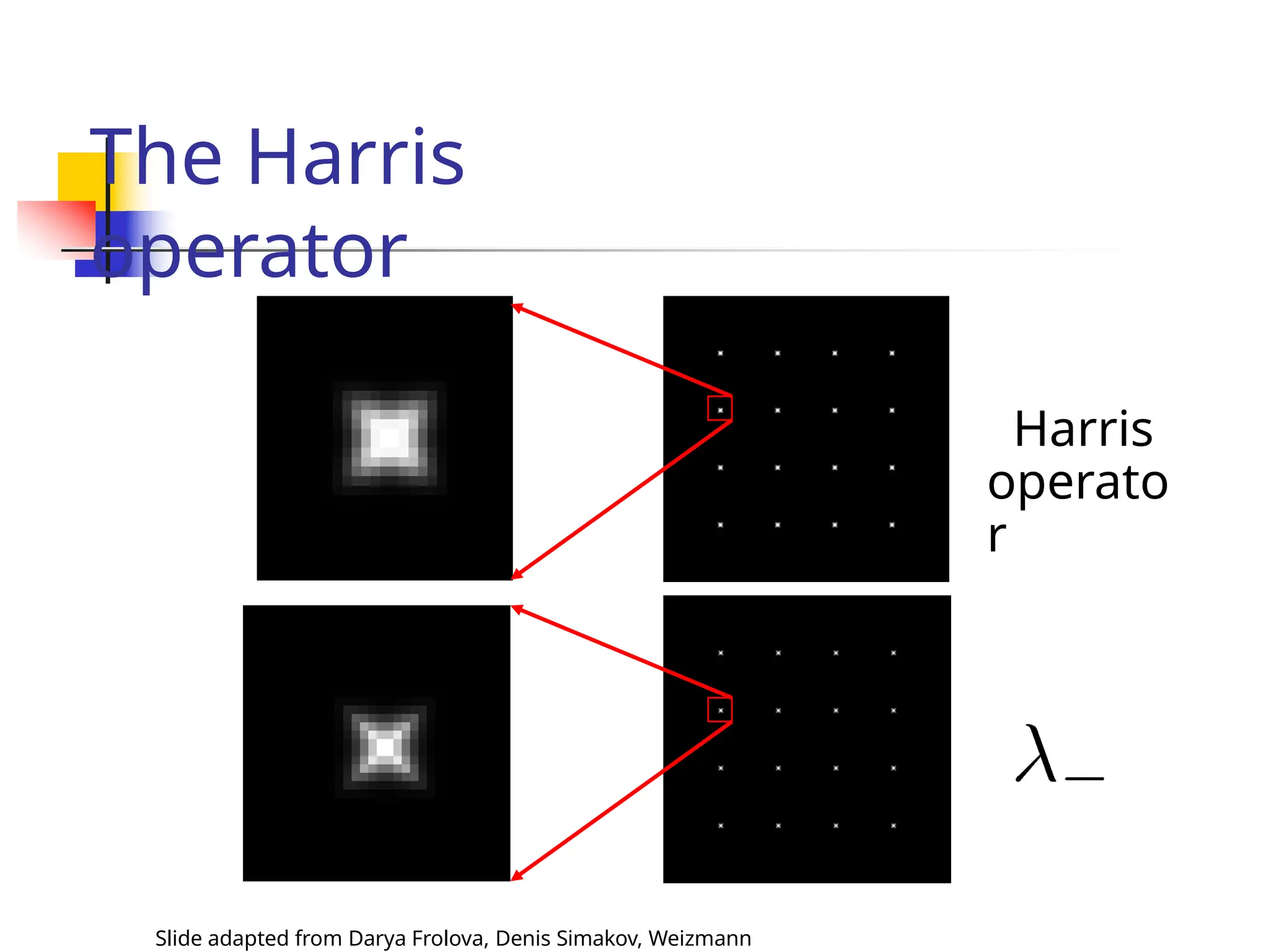
The Harris
operator
- is a variant of the “Harris operator” for feature
detection.
• The trace is the sum of the diagonals, i.e.,
trace(H) = h11 + h22
• Very similar to - but less expensive (no square
root)
• Called the “Harris Corner Detector” or “Harris
The Harris
operator
Harris
operato
r
Slide adapted from Darya Frolova, Denis Simakov, Weizmann
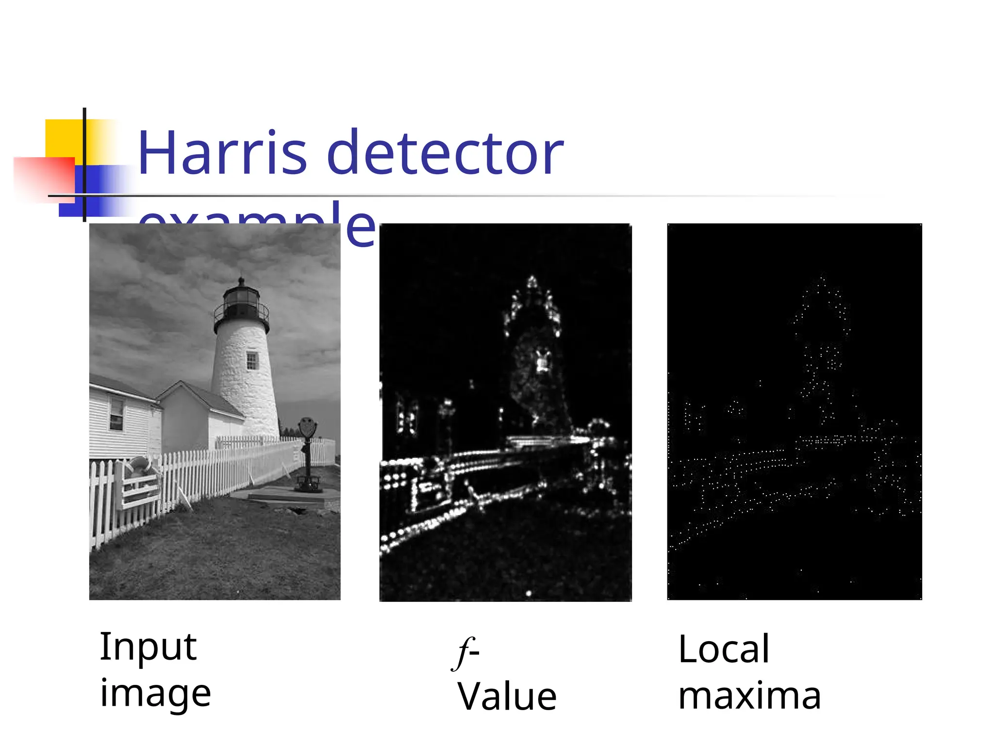
Harris detector
example
Input
image
f-
Value
Local
maxima
Feature
matching
?
Matching with
Features
Slide adapted from Darya Frolova, Denis Simakov, Weizmann
o Detect feature points in both
images.
o Describe them by local statistics.
o Find corresponding pairs
(Matching).
Invarianc
e
Slide adapted from Darya Frolova, Denis Simakov, Weizmann
o
Is it possible to select same features
under various transformations?
o Rotation
o Change of illumination
o Scale
o ..
Scale invariant
detection
Slide adapted from Darya Frolova, Denis Simakov, Weizmann
Key idea for detecting corners
Find scale that gives local maximum of f.

f is a local maximum in both position
and scale

Common definition of f: Laplacian
(or difference between two Gaussian
filtered images with different s.d.’s.).
Invarianc
e
Slide adapted from Darya Frolova, Denis Simakov, Weizmann

Translation

Rotation

Scale

Reflection

Non-uniform
scaling

Illumination

Consider two images I1 and I2 so that I2
is a transformed version of I1

For example,
Tranformational
Invariance:
Detection of the same
features regardless of
the transformation.
Detection and description:
to be invariant
Slide adapted from Darya Frolova, Denis Simakov, Weizmann
Both should be ensured.
1. Detector to be transformational invariant.
 Harris measure is invariant to translation and rotation.
 Scale requires handling of multi-resolution
representation

Usual approach: Computing features at multiple scales
using a Gaussian pyramid.

More precise computation locates features at “the
best scale” (e.g., SIFT)
2. Feature descriptor to be transformational invariant.

captures the information in a region around the
detected feature point.

e.g. histogram of gradient directions in a square window
centering a feature point.
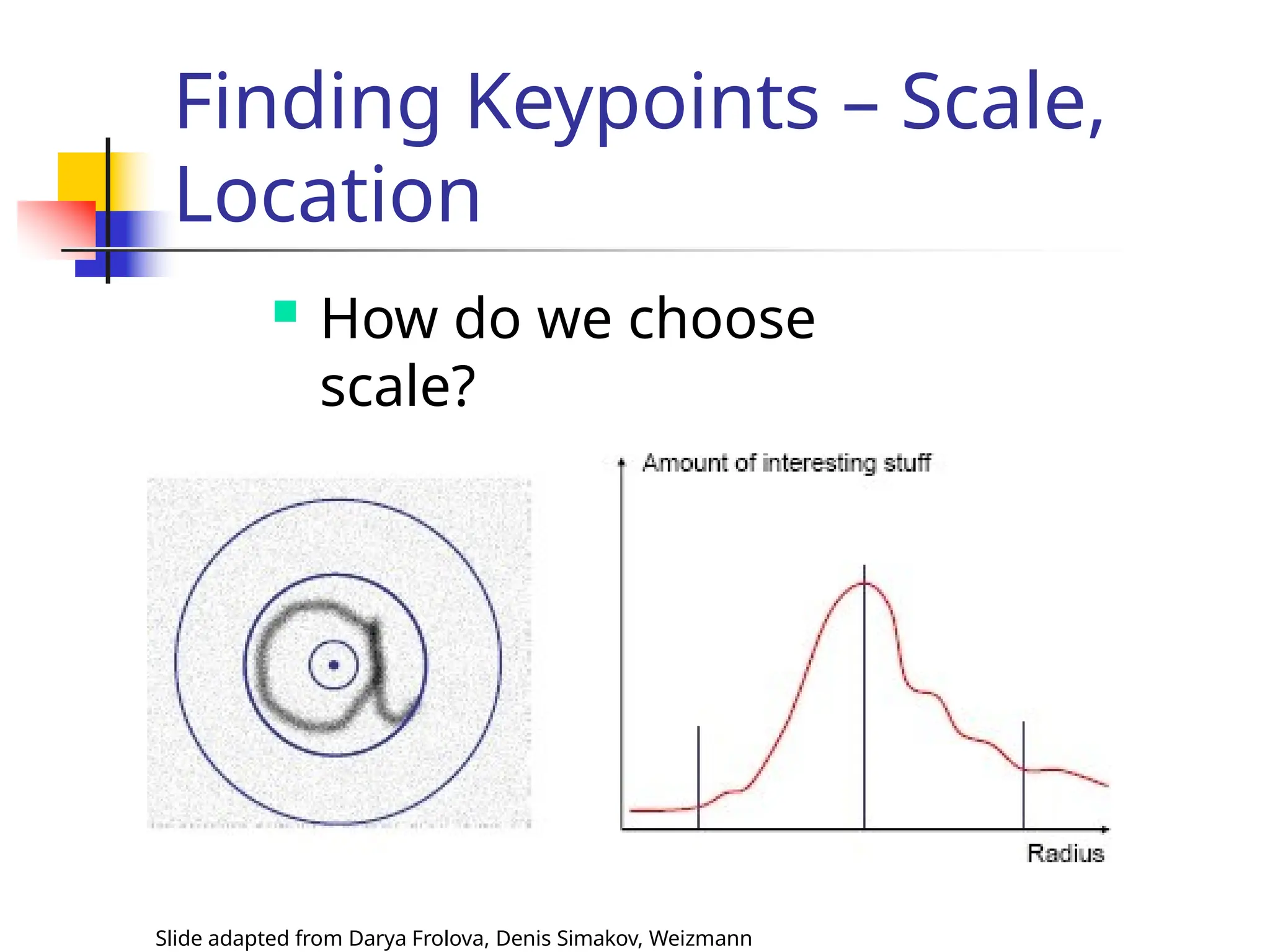
Finding Keypoints – Scale,
Location
 How do we choose
scale?
Slide adapted from Darya Frolova, Denis Simakov, Weizmann
Scale Invariant
Detection
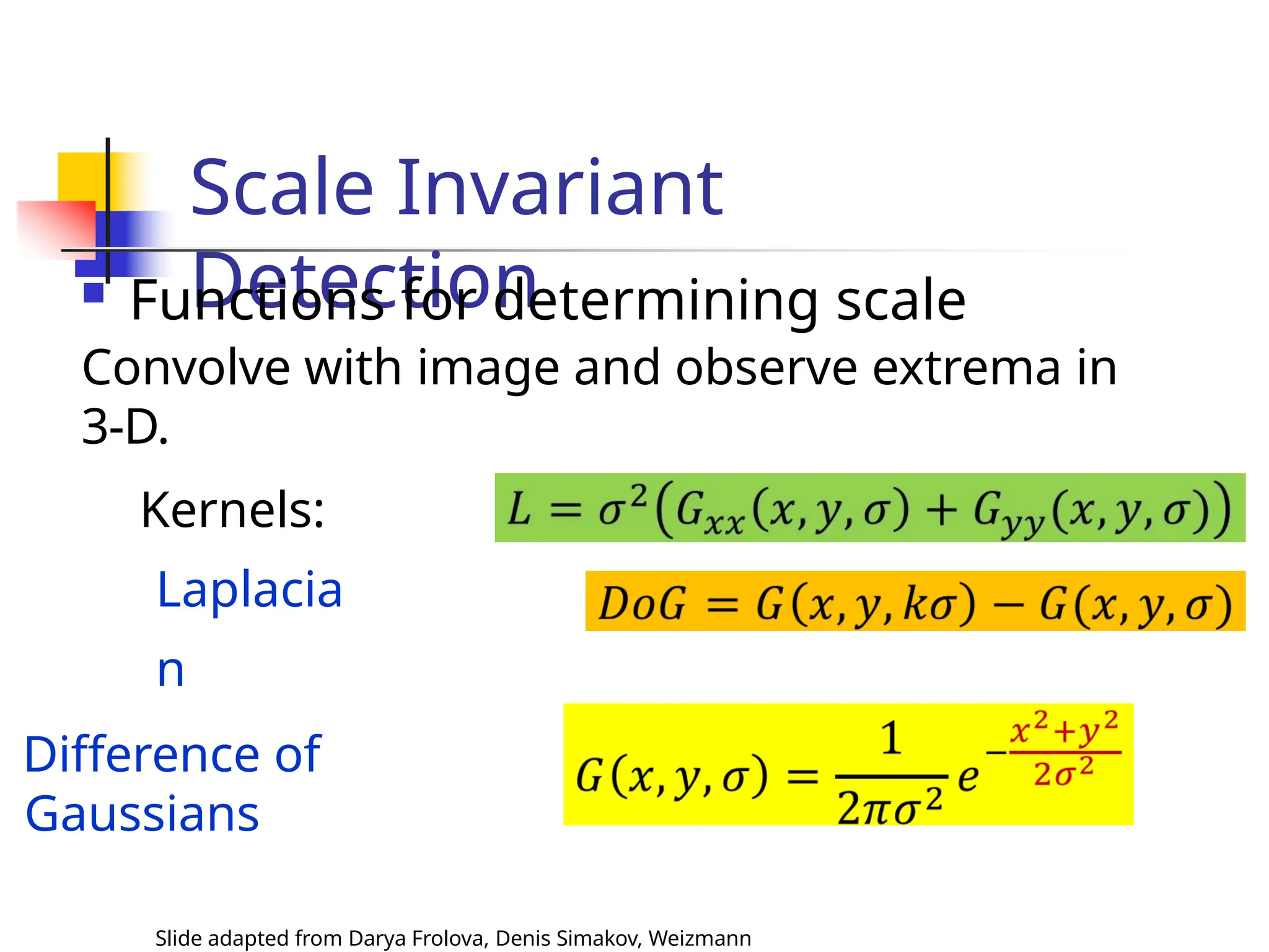
 Functions for determining scale
Convolve with image and observe extrema in
3-D.
Kernels:
Laplacia
n
Difference of
Gaussians
Slide adapted from Darya Frolova, Denis Simakov, Weizmann
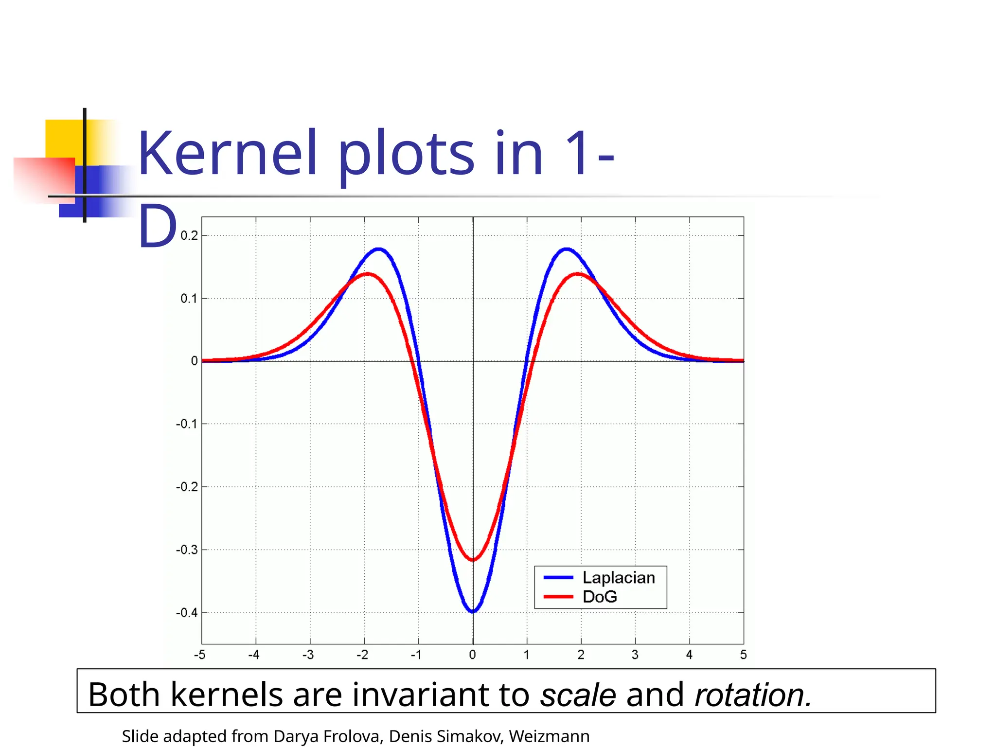
Both kernels are invariant to scale and rotation.
Slide adapted from Darya Frolova, Denis Simakov, Weizmann
Kernel plots in 1-
D
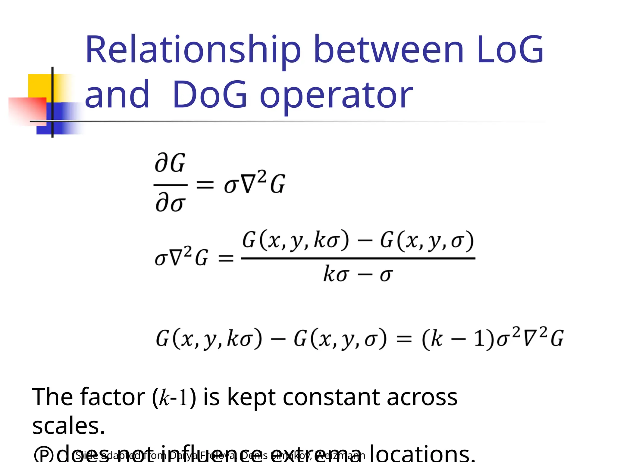
Relationship between LoG
and DoG operator
The factor (k-1) is kept constant across
scales.
Slide adapted from Darya Frolova, Denis Simakov, Weizmann
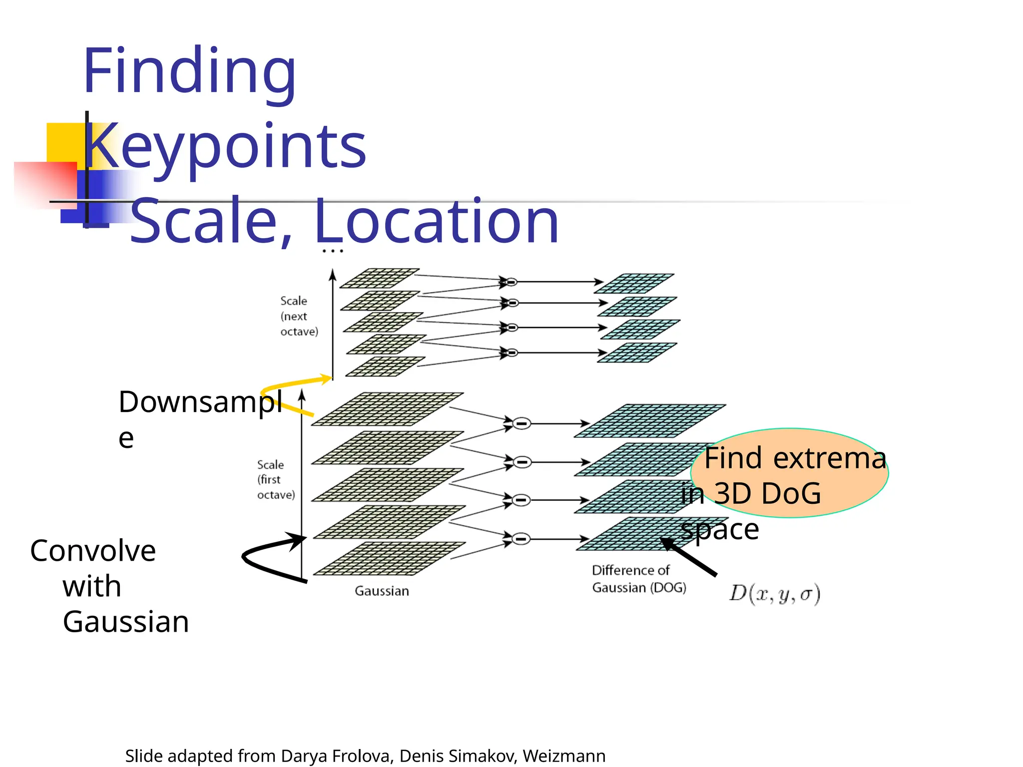
Finding
Keypoints
– Scale, Location
Convolve
with
Gaussian
Downsampl
e
Find extrema
in 3D DoG
space
Slide adapted from Darya Frolova, Denis Simakov, Weizmann
Scale Invariant
Detectors
 Harris-Laplacian (Mikolajczyk & Schmid)

Apply Laplacian operation with varying scale.

Get local maxima of Harris corner response in
space and scale.
• SIFT (Lowe)
• Find local maximum Difference of Gaussians in
space and scale
K. Mikolajczyk, C.Schmid. “Indexing Based on Scale Invariant Interest
Points”. ICCV 2001.
D.Lowe. “Distinctive Image Features from Scale-Invariant Keypoints”.
IJCV 2004
Scale Invariant
Detection: Summary
Slide adapted from Darya Frolova, Denis Simakov, Weizmann
 Given: two images of the same scene with a large
scale difference between them.
 Goal: find the same interest points
independently in each image.
 Solution: search for maxima of suitable
functions in
scale and in space (over the image).
Methods:
1. Harris-Laplacian [Mikolajczyk, Schmid]: maximize
Laplacian over scale, Harris’ measure of corner
response over the image.
Keypoint
localization
Slide adapted from Darya Frolova, Denis Simakov, Weizmann
 There are still a lot of points, some
of them are not good enough.
 The locations of keypoints may be
not accurate.
 Eliminating edge points.
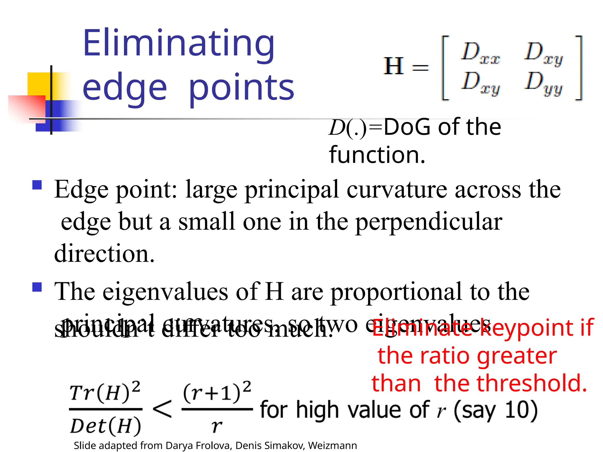
Eliminating
edge points
shouldn’t differ too much.
D(.)=DoG of the
function.
 Edge point: large principal curvature across the
edge but a small one in the perpendicular
direction.
 The eigenvalues of H are proportional to the
principal curvatures, so two eigenvalues
Eliminate keypoint if
the ratio greater
than the threshold.
Slide adapted from Darya Frolova, Denis Simakov, Weizmann
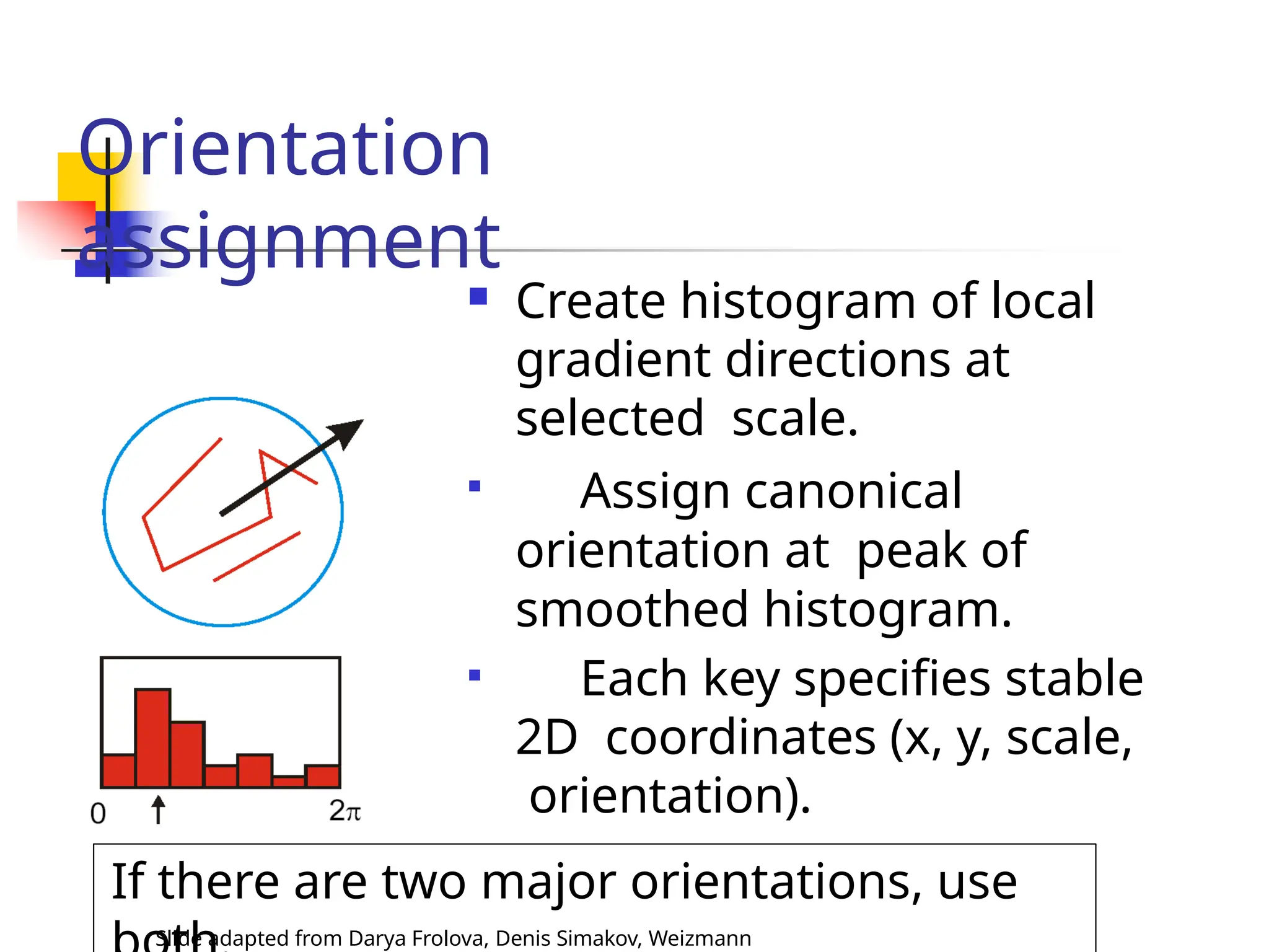
Orientation
assignment
 Create histogram of local
gradient directions at
selected scale.

Assign canonical
orientation at peak of
smoothed histogram.

Each key specifies stable
2D coordinates (x, y, scale,
orientation).
Slide adapted from Darya Frolova, Denis Simakov, Weizmann
If there are two major orientations, use
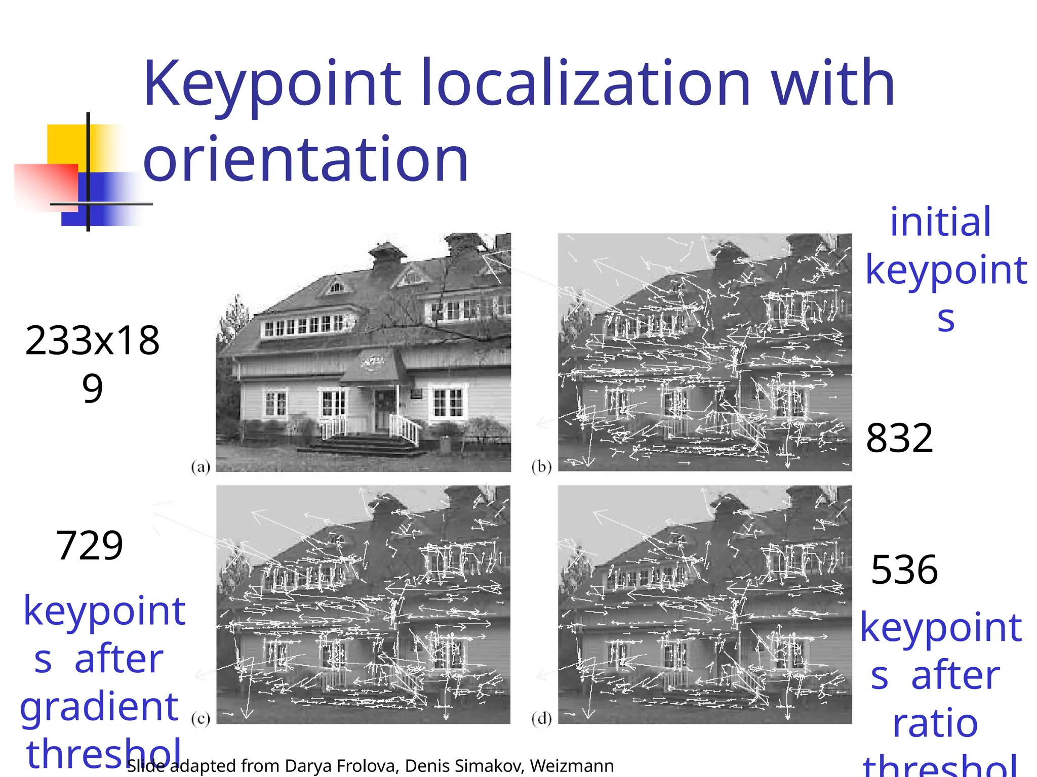
Keypoint localization with
orientation
233x18
9
729
keypoint
s after
gradient
threshol
Slide adapted from Darya Frolova, Denis Simakov, Weizmann
initial
keypoint
s
832
536
keypoint
s after
ratio
Keypoint
Descriptors
 At this point, each keypoint has

location

scale

orientation
 Next is to compute a descriptor for the
local image region about each keypoint
that is

highly distinctive

invariant as possible to variations such
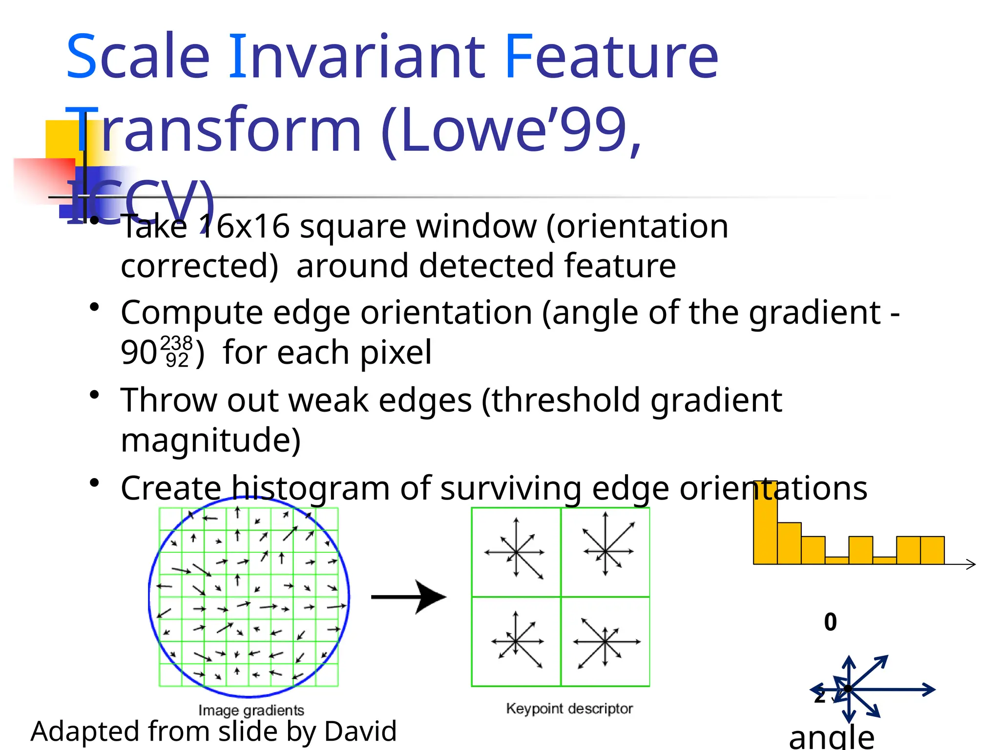
Scale Invariant Feature
Transform (Lowe’99,
ICCV)
• Take 16x16 square window (orientation
corrected) around detected feature
• Compute edge orientation (angle of the gradient -
90) for each pixel
• Throw out weak edges (threshold gradient
magnitude)
• Create histogram of surviving edge orientations
0
2
angle
Adapted from slide by David
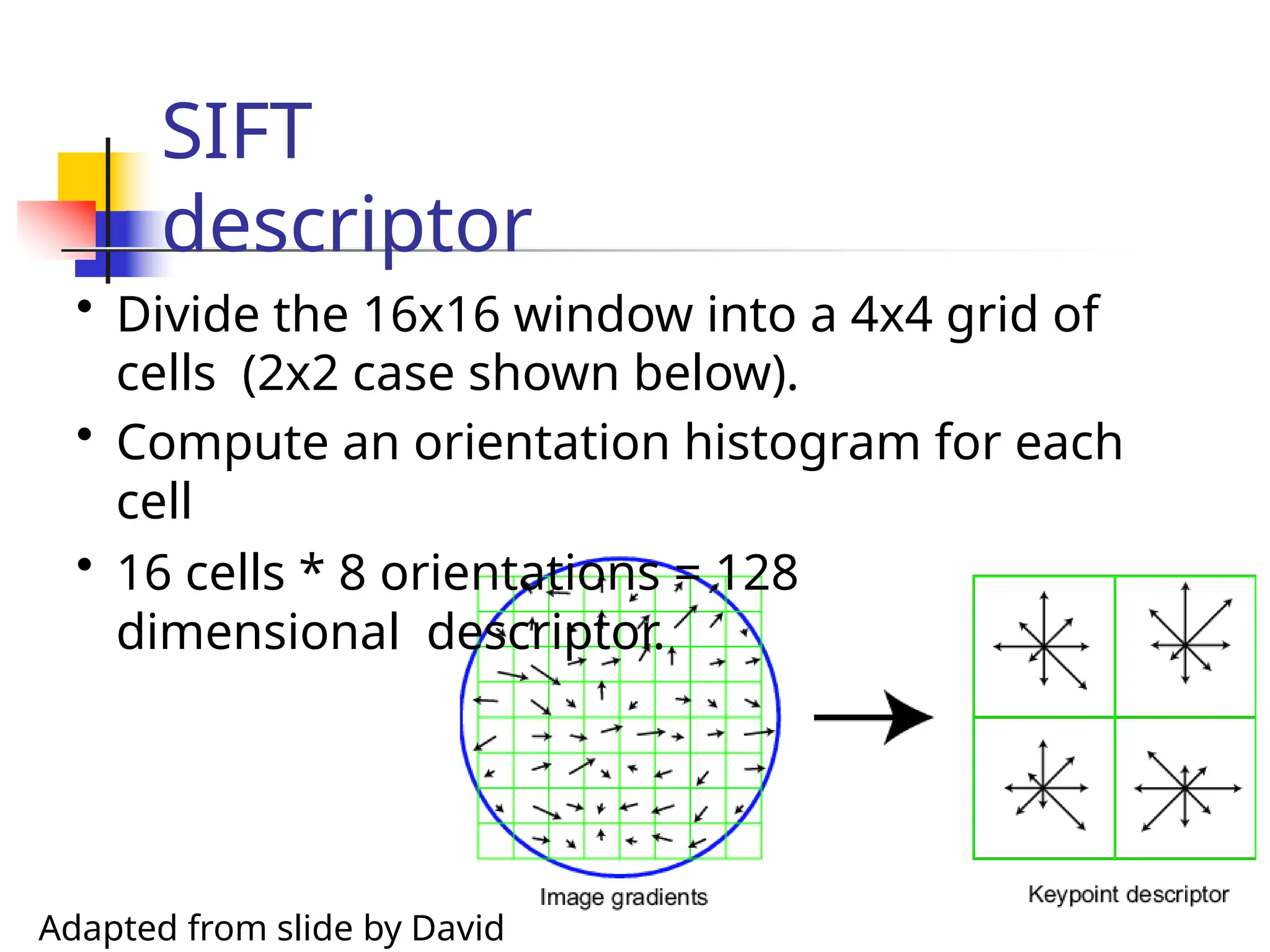
SIFT
descriptor
• Divide the 16x16 window into a 4x4 grid of
cells (2x2 case shown below).
• Compute an orientation histogram for each
cell
• 16 cells * 8 orientations = 128
dimensional descriptor.
Adapted from slide by David
Robustnes
s
Capable of handling

changes in viewpoint

Up to about 60 degree out of plane
rotation

significant changes in illumination

Sometimes even day vs. night
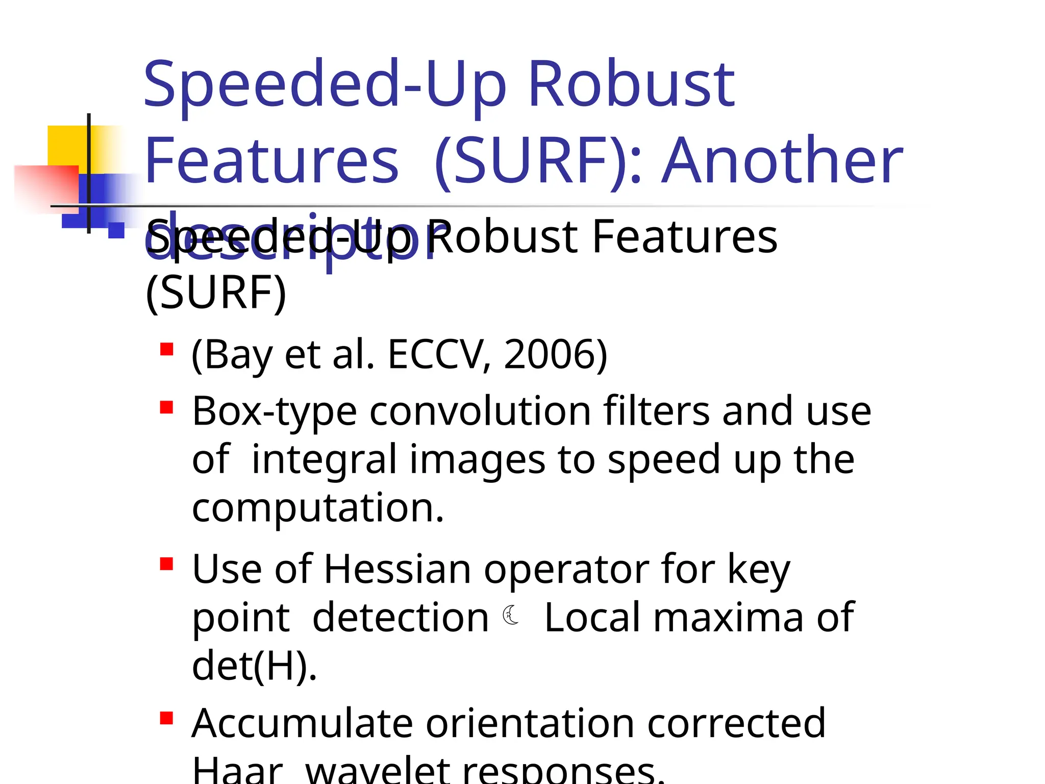
Speeded-Up Robust
Features (SURF): Another
descriptor
 Speeded-Up Robust Features
(SURF)

(Bay et al. ECCV, 2006)
 Box-type convolution filters and use
of integral images to speed up the
computation.

Use of Hessian operator for key
point detection Local maxima of
det(H).

Accumulate orientation corrected
Hessian
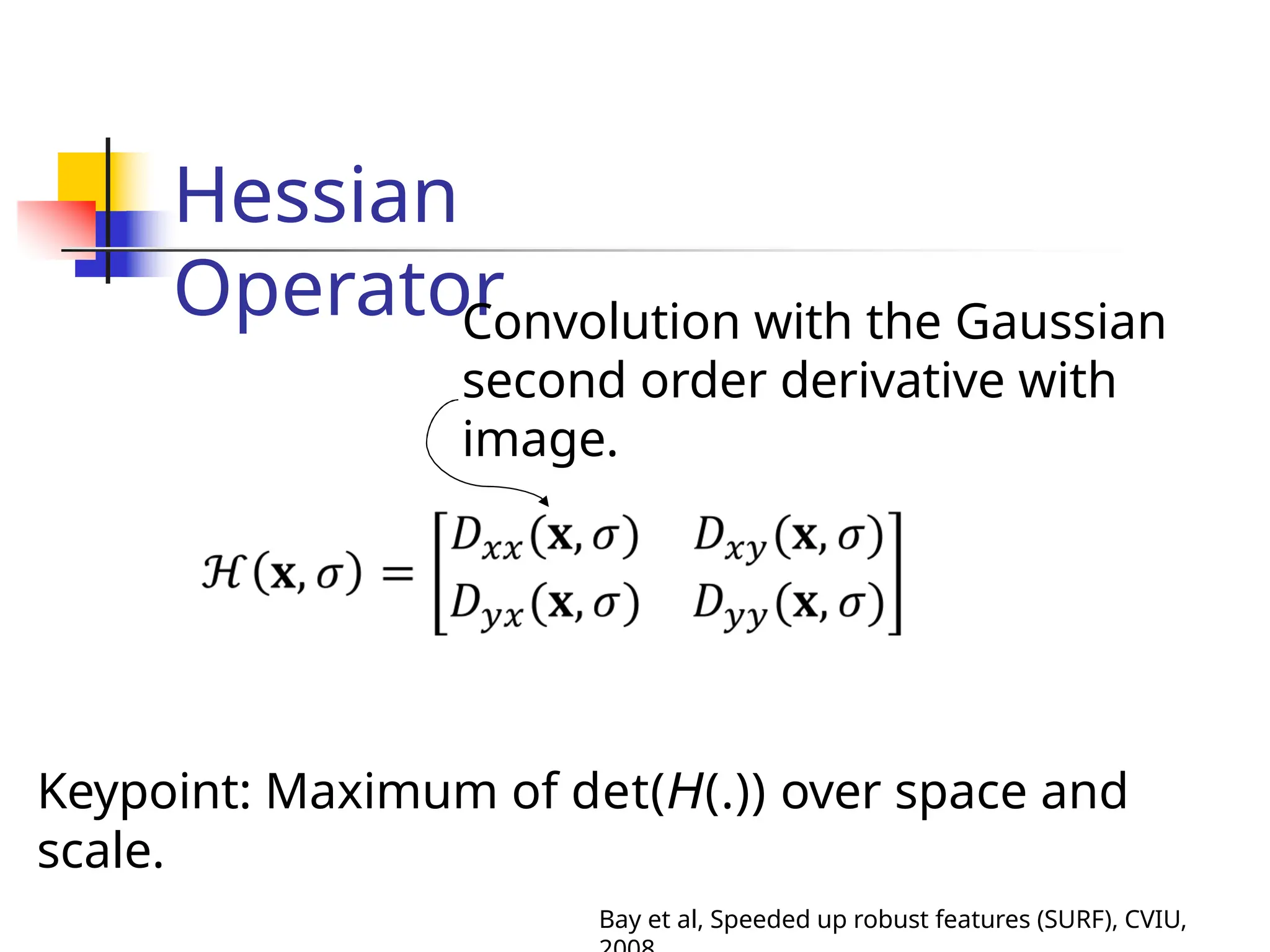
Operator
Convolution with the Gaussian
second order derivative with
image.
Keypoint: Maximum of det(H(.)) over space and
scale.
Bay et al, Speeded up robust features (SURF), CVIU,
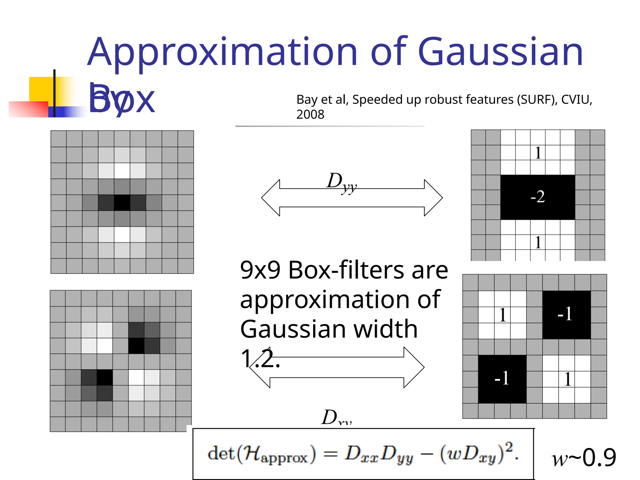
Approximation of Gaussian
by
Box
filters
Dxy
Dyy
9x9 Box-filters are
approximation of
Gaussian width
1.2.
w~0.9
Bay et al, Speeded up robust features (SURF), CVIU,
2008
Fast computation using the
integral image
Only 3
additions and
four memory
access.
Bay et al, Speeded up robust features (SURF), CVIU,
2008
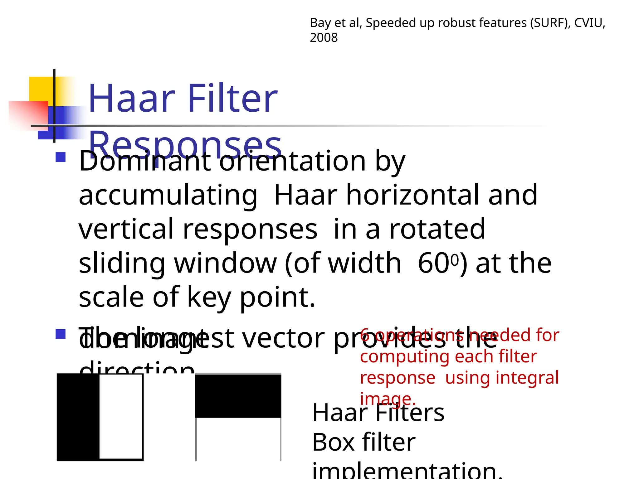
Haar Filter
Responses
 Dominant orientation by
accumulating Haar horizontal and
vertical responses in a rotated
sliding window (of width 600) at the
scale of key point.
 The longest vector provides the
dominant
direction.
Haar Filters
Box filter
Bay et al, Speeded up robust features (SURF), CVIU,
2008
6 operations needed for
computing each filter
response using integral
image.
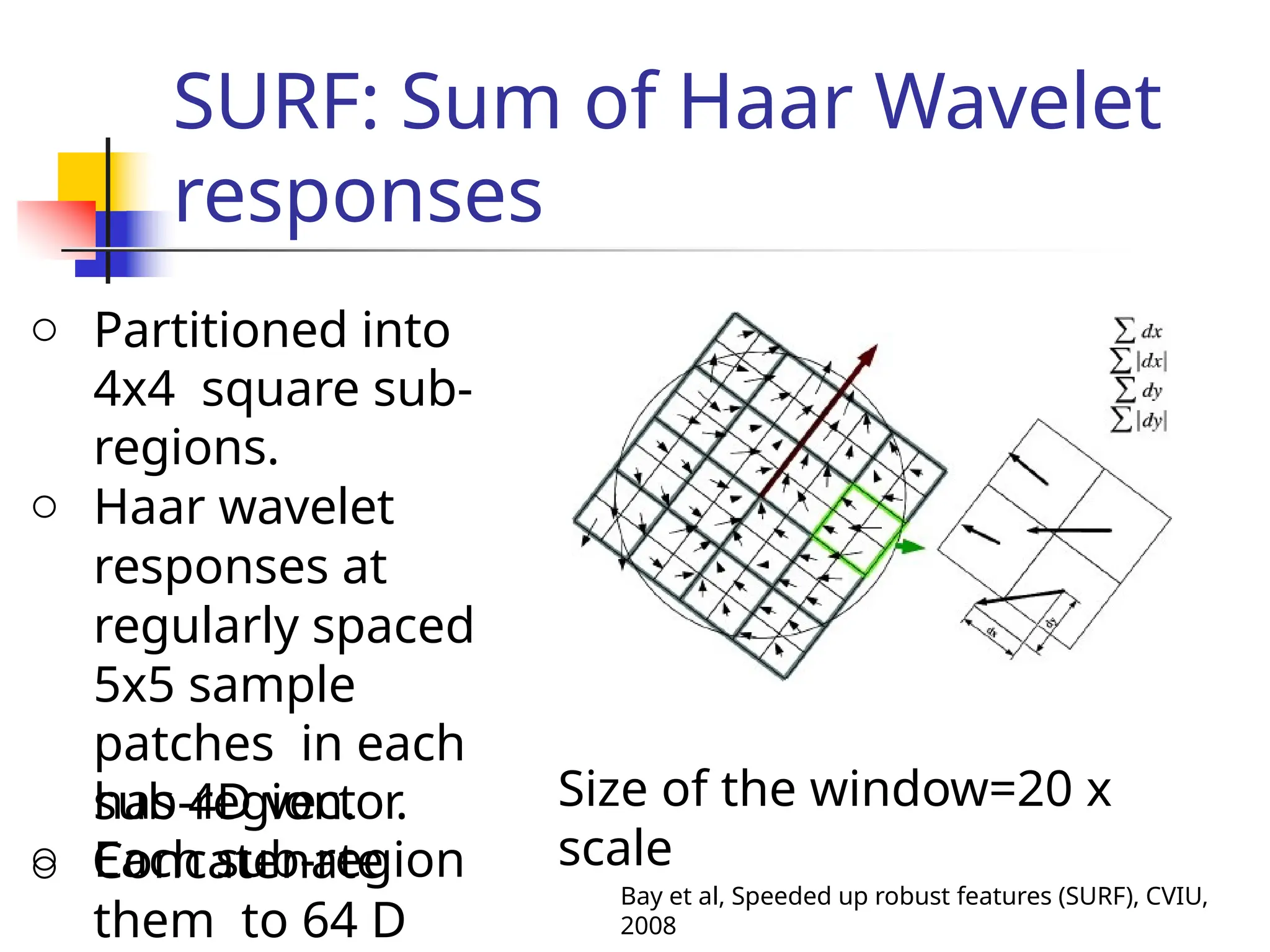
SURF: Sum of Haar Wavelet
responses
Size of the window=20 x
scale
o Partitioned into
4x4 square sub-
regions.
o Haar wavelet
responses at
regularly spaced
5x5 sample
patches in each
sub-region.
o Each sub-region
has 4D vector.
o Concatenate
them to 64 D
Bay et al, Speeded up robust features (SURF), CVIU,
2008
Other types of detectors and
descriptors
 FAST: Features from Accelerated
Segment Test (Rosten et al,
PAMI, 2010).
 BRIEF: Binary Robust Independent
Elementary Features (Colonder et
al, ECCV, 2010).
 ORB: Oriented FAST and Rotated
BRIEF (Rublee et al, ICCV, 2011)
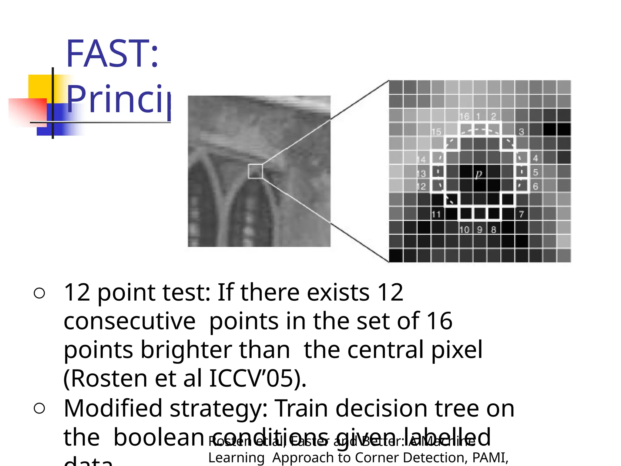
FAST:
Principle
o 12 point test: If there exists 12
consecutive points in the set of 16
points brighter than the central pixel
(Rosten et al ICCV’05).
o Modified strategy: Train decision tree on
the boolean conditions given labelled
Rosten et al, Faster and Better: A Machine
Learning Approach to Corner Detection, PAMI,
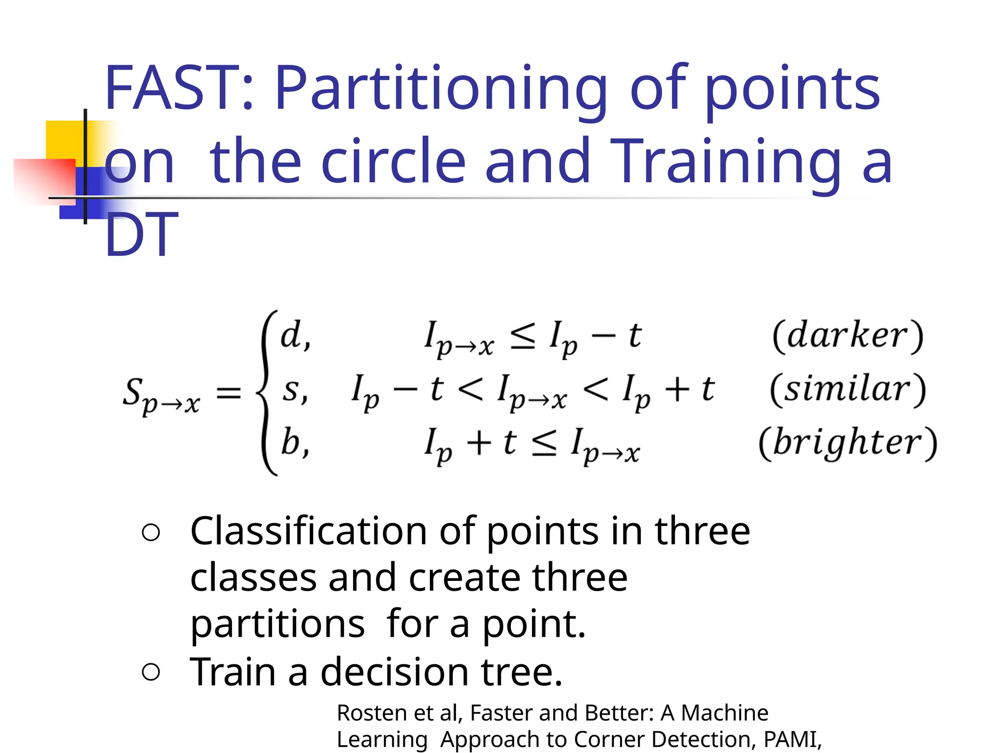
FAST: Partitioning of points
on the circle and Training a
DT
o Classification of points in three
classes and create three
partitions for a point.
o Train a decision tree.
Rosten et al, Faster and Better: A Machine
Learning Approach to Corner Detection, PAMI,
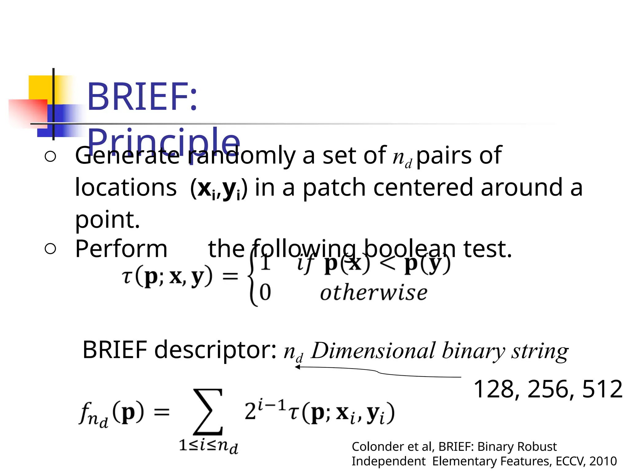
BRIEF:
Principle
o Generate randomly a set of nd pairs of
locations (xi,yi) in a patch centered around a
point.
o Perform the following boolean test.
BRIEF descriptor: nd Dimensional binary string
128, 256, 512
Colonder et al, BRIEF: Binary Robust
Independent Elementary Features, ECCV, 2010
ORB(Oriented FAST and
rotated BRIEF): Principle
 FAST does not operate across scale.
 Apply FAST detector on pyramid
of smoothened images.
 Orientation by intensity centroid: The
vector from the center of the patch and to
a centroid considering the intensity
distribution (intensity weighted center of
patch).
 Rotate the patch by the angle and
Matchin
g
 Representation of a key-point by a feature
vector.
 e.g. [f0 f1 … fn]T
 Use distance functions / similarity measures.
 L1 norm
 L2
norm
 L
Region
descriptors
 Patch descriptors
 Texture descriptors
 Image / Sub-Image global
descriptors
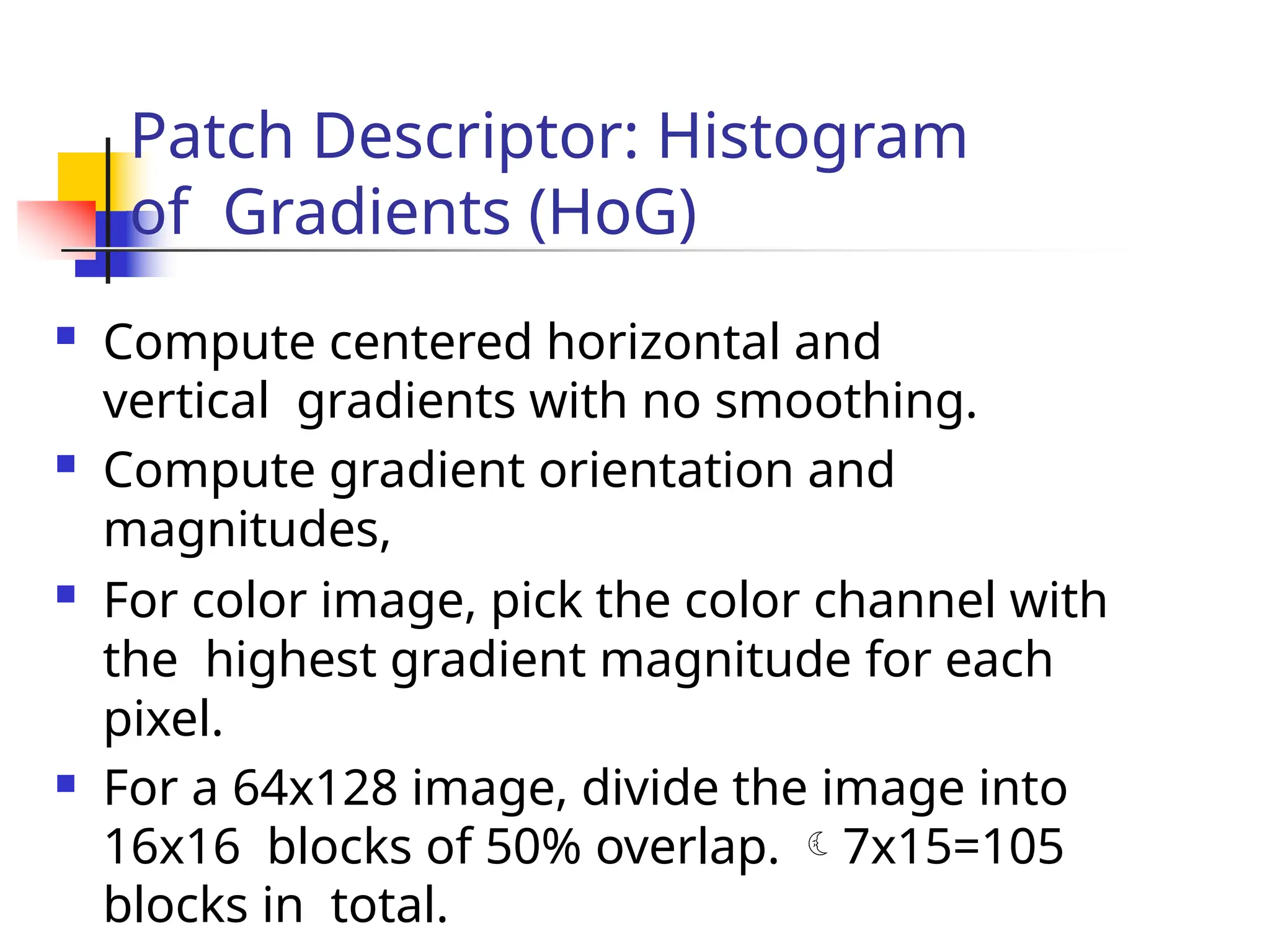
Patch Descriptor: Histogram
of Gradients (HoG)
 Compute centered horizontal and
vertical gradients with no smoothing.
 Compute gradient orientation and
magnitudes,
 For color image, pick the color channel with
the highest gradient magnitude for each
pixel.
 For a 64x128 image, divide the image into
16x16 blocks of 50% overlap. 7x15=105
blocks in total.
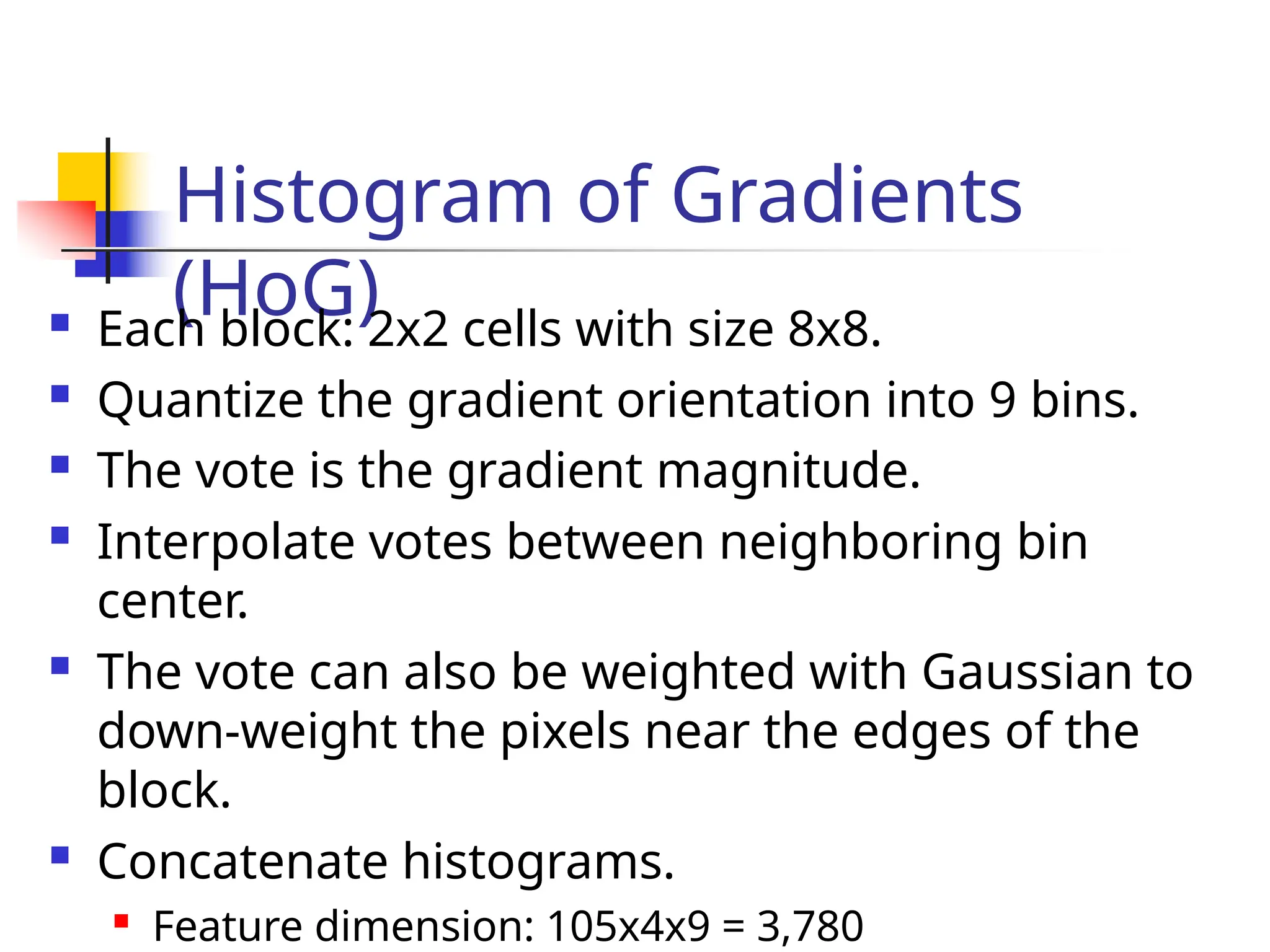
Histogram of Gradients
(HoG)
 Each block: 2x2 cells with size 8x8.
 Quantize the gradient orientation into 9 bins.
 The vote is the gradient magnitude.
 Interpolate votes between neighboring bin
center.
 The vote can also be weighted with Gaussian to
down-weight the pixels near the edges of the
block.
 Concatenate histograms.

Feature dimension: 105x4x9 = 3,780
Object detection with
patch descriptors.
 Typical examples:

Pedestrian detection

Character recognition
 Detection as a classification task.

Generate labeled sample feature
descriptors.

Train a classifier.

NN, SVM, Decision Tree, Random Forest …..

Label an unknown patch using its
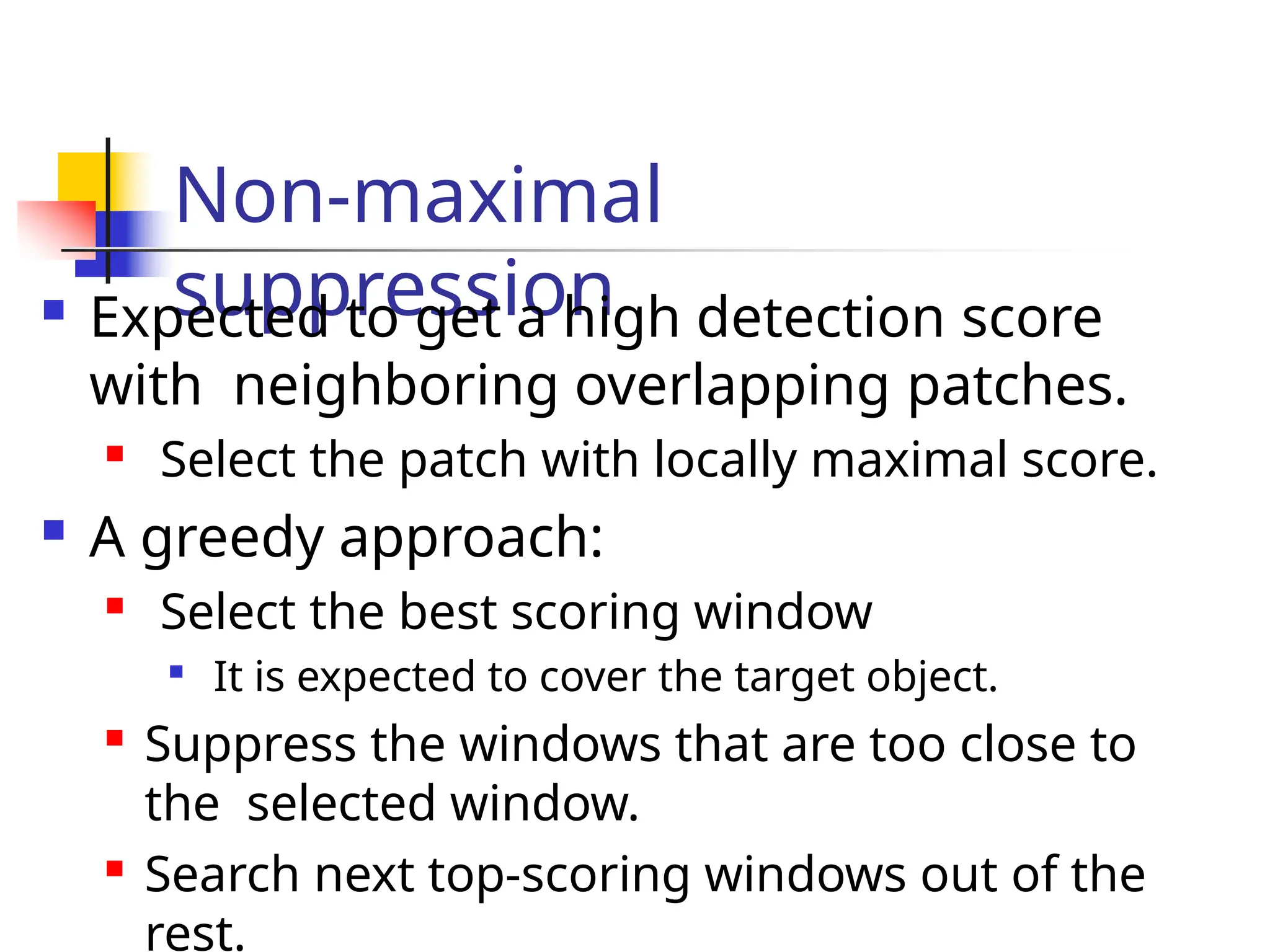
Non-maximal
suppression
 Expected to get a high detection score
with neighboring overlapping patches.

Select the patch with locally maximal score.
 A greedy approach:

Select the best scoring window

It is expected to cover the target object.

Suppress the windows that are too close to
the selected window.

Search next top-scoring windows out of the
rest.
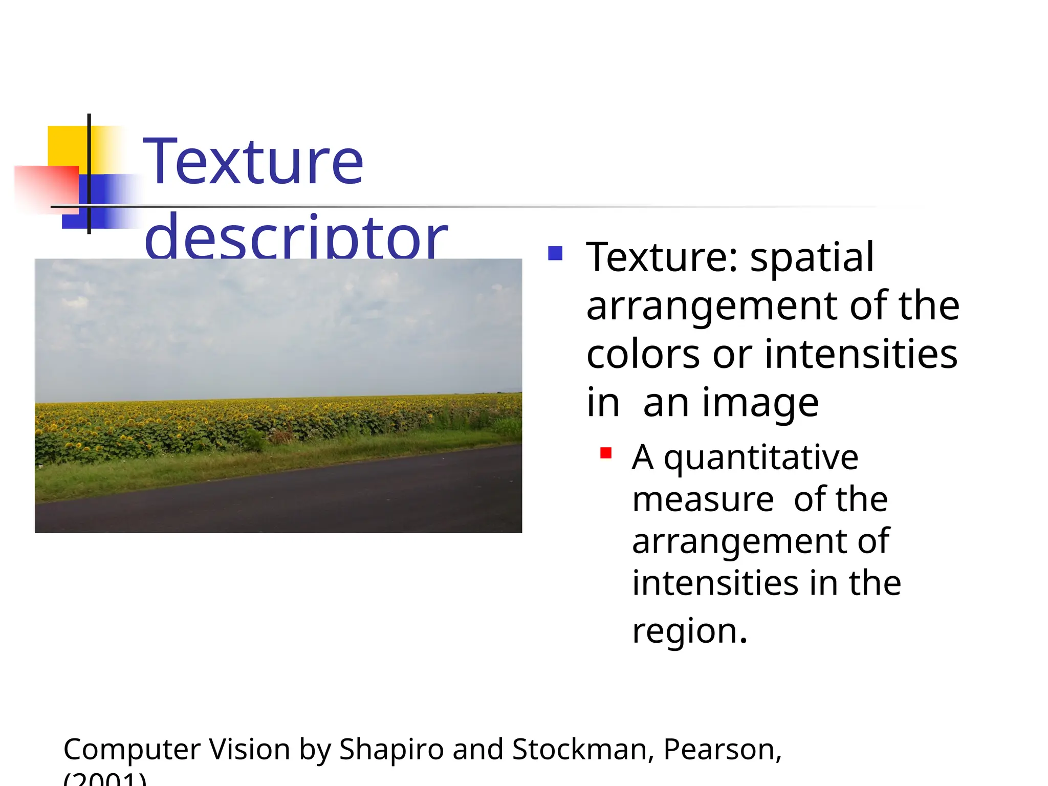
Texture
descriptor  Texture: spatial
arrangement of the
colors or intensities
in an image
 A quantitative
measure of the
arrangement of
intensities in the
region.
Computer Vision by Shapiro and Stockman, Pearson,
Texture
descriptors
 Edge density and direction
 Local Binary Pattern (LBP).
 Co-occurrence Matrix.
 Laws’ texture energy
features.
Edge density and
direction
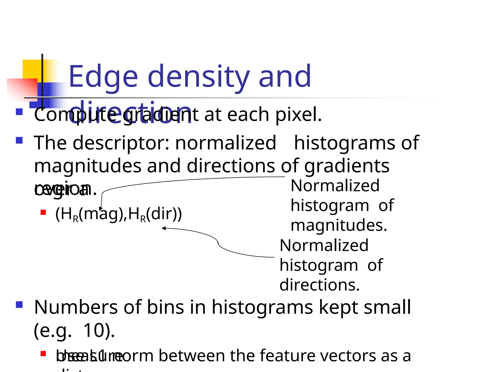
 Compute gradient at each pixel.
 The descriptor: normalized histograms of
magnitudes and directions of gradients
over a
region.
 (HR(mag),HR(dir))
measure
Normalized
histogram of
directions.
 Numbers of bins in histograms kept small
(e.g. 10).

Use L1 norm between the feature vectors as a
Normalized
histogram of
magnitudes.
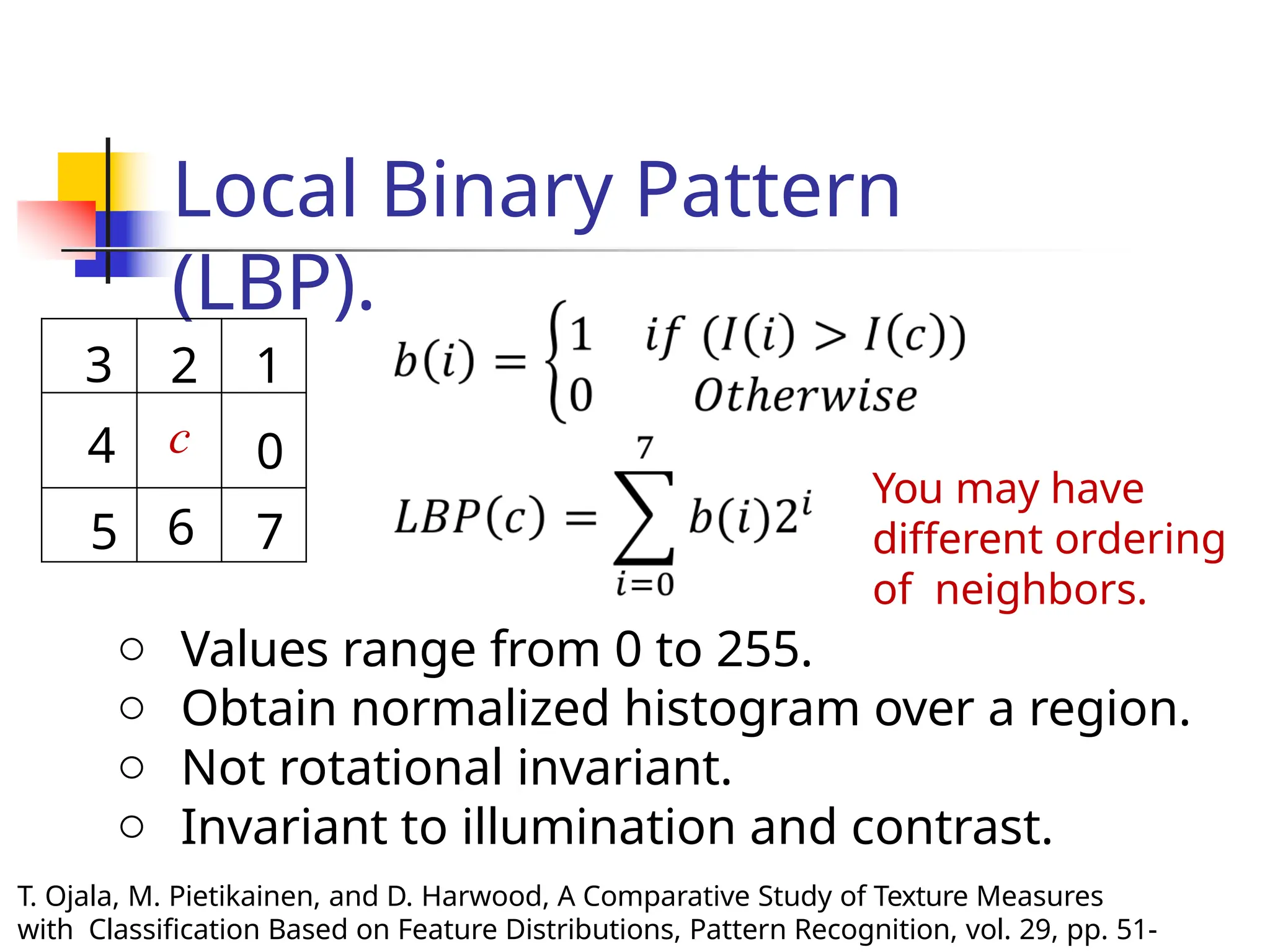
Local Binary Pattern
(LBP).
3 2 1
4 c 0
5 6 7
You may have
different ordering
of neighbors.
o Values range from 0 to 255.
o Obtain normalized histogram over a region.
o Not rotational invariant.
o Invariant to illumination and contrast.
T. Ojala, M. Pietikainen, and D. Harwood, A Comparative Study of Texture Measures
with Classification Based on Feature Distributions, Pattern Recognition, vol. 29, pp. 51-
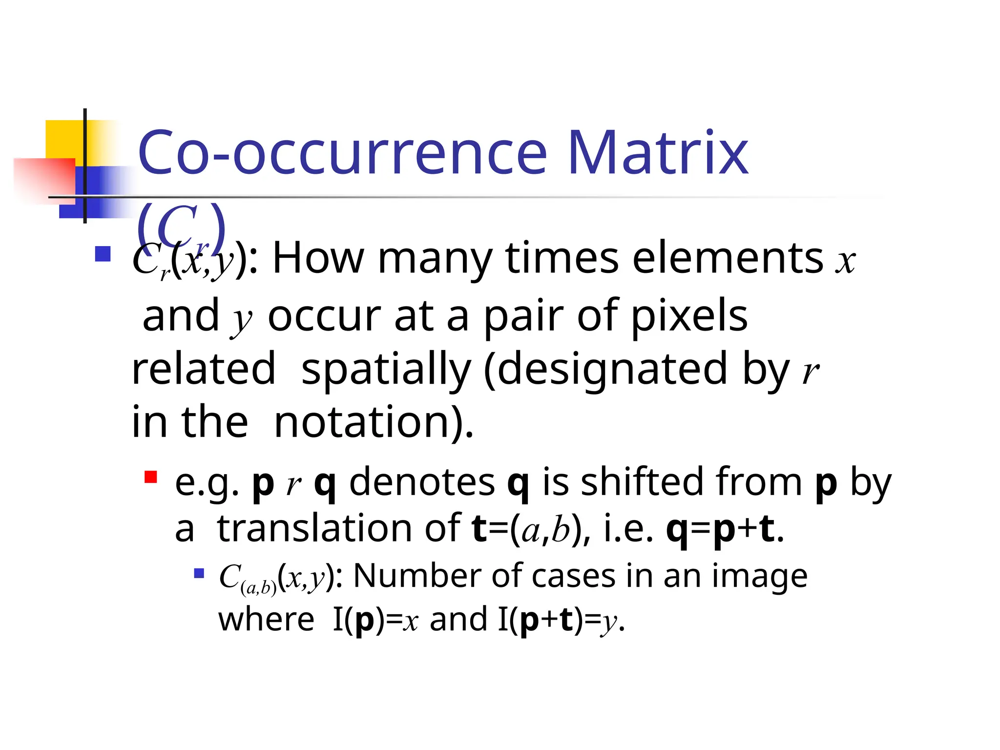
Co-occurrence Matrix
(Cr)
 Cr(x,y): How many times elements x
and y occur at a pair of pixels
related spatially (designated by r
in the notation).

e.g. p r q denotes q is shifted from p by
a translation of t=(a,b), i.e. q=p+t.
 C(a,b)(x,y): Number of cases in an image
where I(p)=x and I(p+t)=y.
Laws’ texture energy
features
 A set of 9 5x5 masks used to
compute
texture energy.
L5 (Level): [1 4 6 4 1]
E5 (Edge): [-1 -2 0 2 1]
S5 (Spot): [-1 0 2 0 -1]
R5 (ripple): [1 -4 6 -4 1]
Computation with
mask: Convolution
A mask: Outer
product of any
pair.
e.g. E5L5: E5.L5T
K. Laws, “Rapid Texture Identification”, in SPIE Vol. 238: Image Processing
for
Laws’ texture energy
features
K. Laws, “Rapid Texture Identification”, in SPIE Vol. 238: Image Processing
for
 A set of 9 5x5 masks used to
compute
texture energy.
L5 (Level): [1 4 6 4 1]
E5 (Edge): [-1 -2 0 2 1]
S5 (Spot): [-1 0 2 0 -1]
R5 (ripple): [1 -4 6 -4 1]
16 such masks possible.
Combine a few pairs to make 9
masks.
L5E5 and E5L5
L5R5 and
R5L5 E5S5
and S5E5
L5S5 and S5L5
E5R5 and
R5E5 S5R5
and R5S5
S5S5
R5R
5
E5E5
Take
average
of
response
s of two
masks.
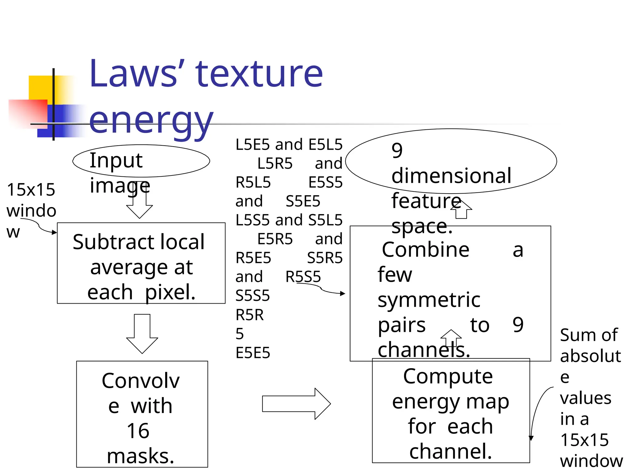
Laws’ texture
energy
Subtract local
average at
each pixel.
Convolv
e with
16
masks.
Compute
energy map
for each
channel.
Combine a
few
symmetric
pairs to 9
channels.
Input
image
9
dimensional
feature
space.
15x15
windo
w
Sum of
absolut
e
values
in a
15x15
window
L5E5 and E5L5
L5R5 and
R5L5 E5S5
and S5E5
L5S5 and S5L5
E5R5 and
R5E5 S5R5
and R5S5
S5S5
R5R
5
E5E5
Use of texture
descriptors
 Detection of object patches
represented by textured
patterns.
 Segmentation of images.
 Classification / Matching

Generate a Library of labelled
feature descriptors.

Detection of classes (class labels).

Matching to the nearest texture
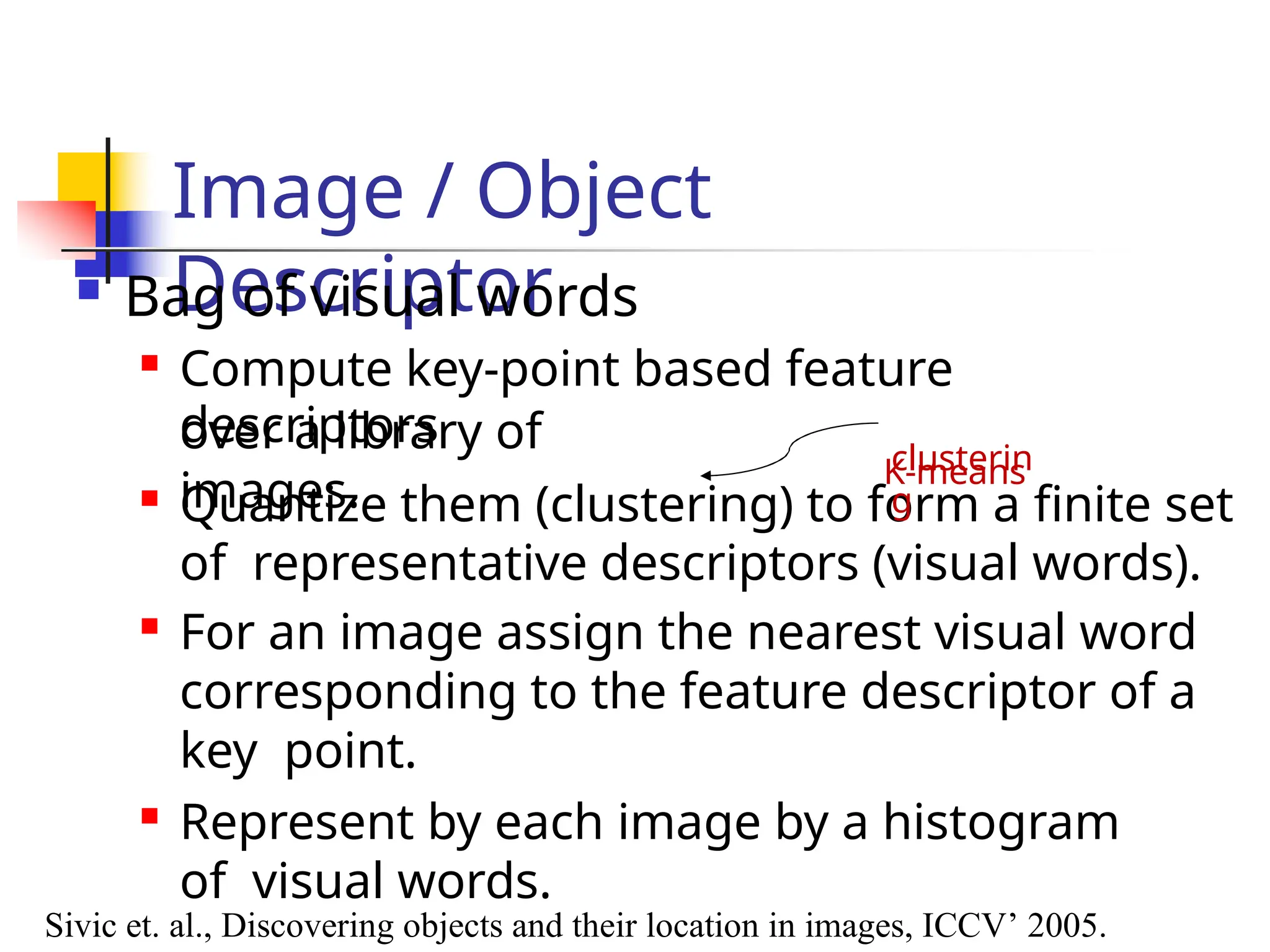
Image / Object
Descriptor
over a library of
images.

Quantize them (clustering) to form a finite set
of representative descriptors (visual words).

For an image assign the nearest visual word
corresponding to the feature descriptor of a
key point.

Represent by each image by a histogram
of visual words.
Sivic et. al., Discovering objects and their location in images, ICCV’ 2005.
 Bag of visual words

Compute key-point based feature
descriptors
K-means
clusterin
g
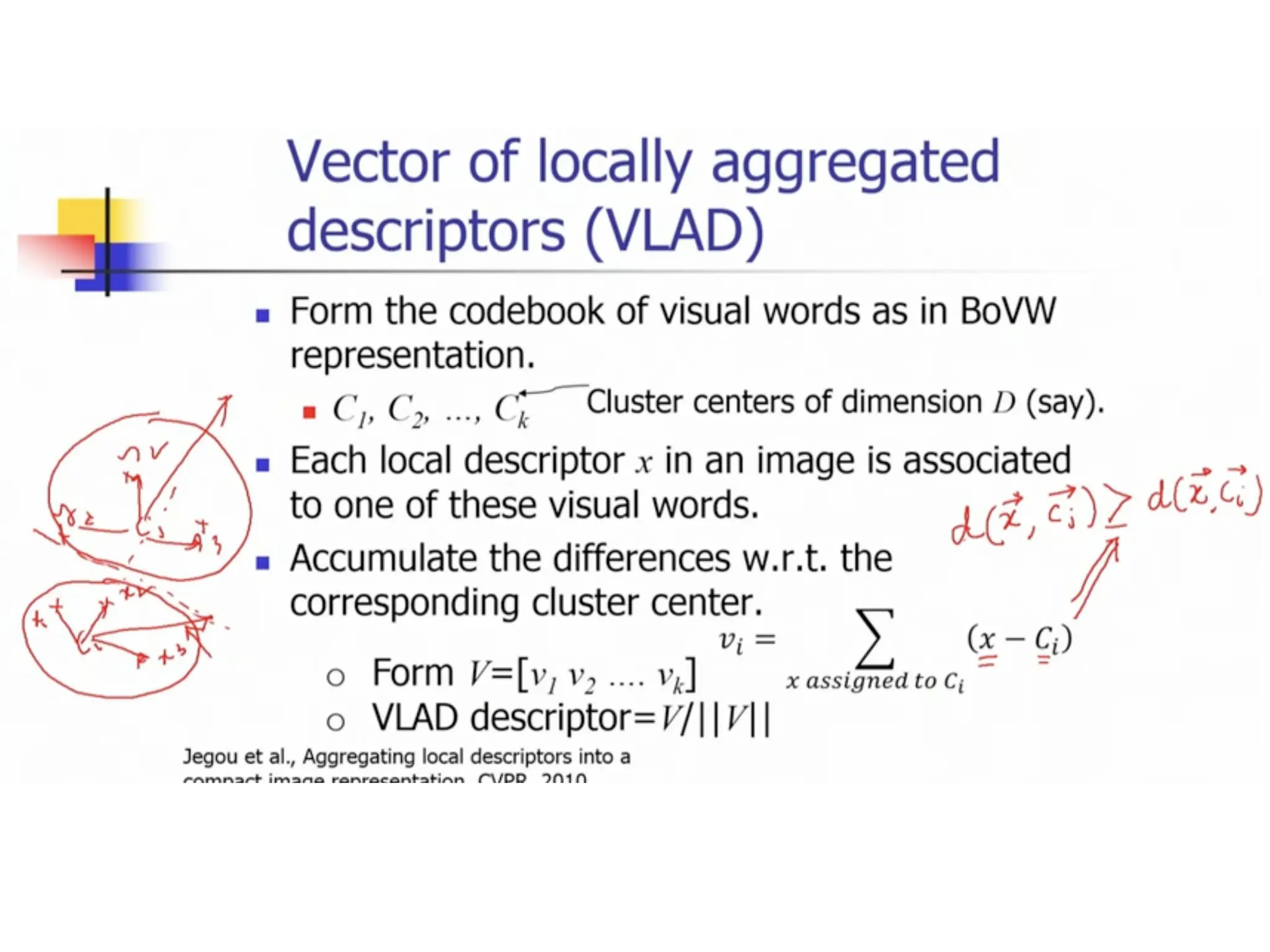
Vector of locally aggregated
descriptors (VLAD)
 Form the codebook of visual words as in
BoVW representation.
 C1, C2, …, Ck
Cluster centers of dimension D
(say).
 Each local descriptor x in an image is
associated to one of these visual words.
 Accumulate the differences w.r.t.
the corresponding cluster center.
o Form V=[v1 v2 …. vk]
o VLAD descriptor=V/||V||
Dimension:
k.D
Jegou et al., Aggregating local descriptors
into a compact image representation, CVPR,
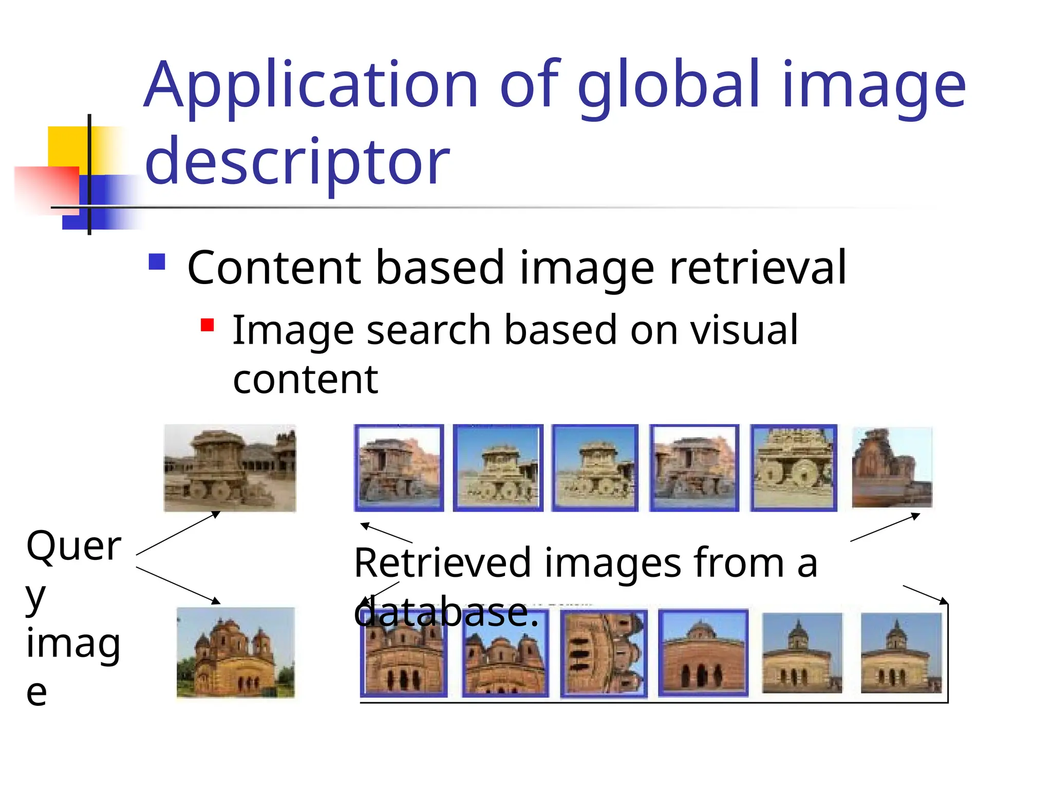
Application of global image
descriptor
 Content based image retrieval

Image search based on visual
content
Quer
y
imag
e
Retrieved images from a
database.
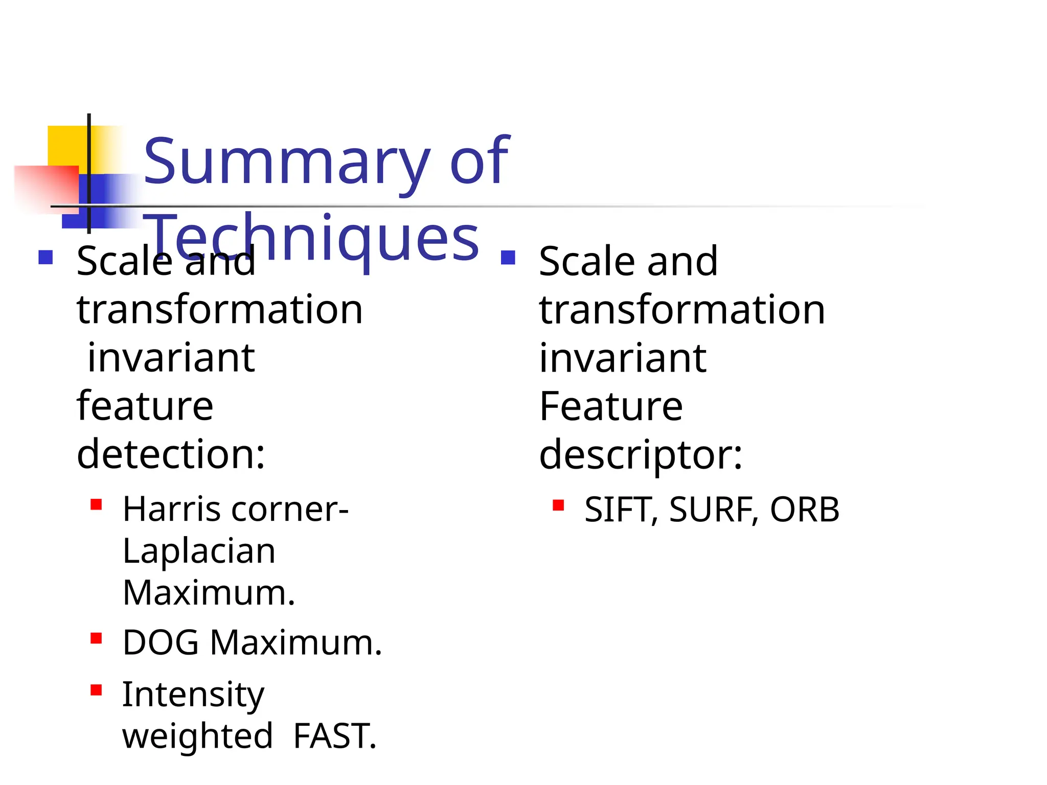
Summary of
Techniques
 Scale and
transformation
invariant
feature
detection:

Harris corner-
Laplacian
Maximum.
 DOG Maximum.
 Intensity
weighted FAST.
 Scale and
transformation
invariant
Feature
descriptor:
 SIFT, SURF, ORB
Summary of
Techniques
 Region and
texture
descriptors.
 HoG
 Edge
density
 LBP

Co-occurrence
matrix
 Laws’ texture
energy
 Image global
descriptor

BoVW

 A few
applications

Key point descriptor:
Matching
corresponding points
of a scene.
 Region
descriptor:
Object detection
 Global
descriptor :Image
retrieval.

feature matching and model description .pptx

  • 1.
  • 2.
    Can you matchthe scene points? o Detection o Descriptio n o Matching
  • 3.
    Feature detection “flat” region: no change in all directions Slideadapted from Darya Frolova, Denis Simakov, Weizmann “edge”: no change along the edge direction “corner”: significant change in all directions A local measure for uniquely identifying the feature.  How does the measure change on shifting windows at different points?
  • 4.
    • compare eachpixel before and after by summing up the squared differences (SSD). • this defines an SSD “error” of E(u,v). Feature detection Consider shifting the window W by (u,v). • how do the pixels in W change? W Slide adapted from Darya Frolova, Denis Simakov, Weizmann
  • 5.
    Small motion assumption For smallu and v Slide adapted from Darya Frolova, Denis Simakov, Weizmann
  • 6.
    Feature detection W                    I I u I  u v I u  v u   I   I v II  y y x x I  x y  u vI x  I x y   u  T  x y   x y I 2   y  2 Slide adapted from Darya Frolova, Denis Simakov, Weizmann
  • 7.
    Feature detection For the exampleabove • Suppose the center of the green window moved to anywhere on the blue unit circle. • Directions for the largest and the smallest E values? • Eigenvectors of H. Slide adapted from Darya Frolova, Denis Simakov, Weizmann
  • 8.
    Quick eigenvalue/eigenvector review The eigenvectors ofa matrix A are the vectors x that satisfy: The scalar  is the eigenvalue corresponding to x  The eigenvalues are found by solving:  For eigen vector solve the following: Once you know , you find eigen vector [x y]T by solving the above Slide adapted from Darya Frolova, Denis Simakov, Weizmann
  • 9.
    Feature detection Eigenvalues and eigenvectorsof H • Define shifts with the smallest and largest change (E value) • x+ = direction of largest increase in E. • + = amount of increase in direction x+ x- x+ Slide adapted from Darya Frolova, Denis Simakov, Weizmann
  • 10.
    Feature scoring function Slide adaptedfrom Darya Frolova, Denis Simakov, Weizmann E(u,v) to be large for small shifts in all directions • the minimum of E(u,v) should be large, over all unit vectors [u v]. • this minimum is given by the smaller eigenvalue (-) of H
  • 11.
    Feature detection Slide adapted fromDarya Frolova, Denis Simakov, Weizmann
  • 12.
    Feature detection: Algorithm • Computethe gradient at each point in the image. • Obtain the H matrix from the entries in the gradient. • Compute eigenvalues of H. • Locate points with large response (- > threshold) • Select points where - is a local maximum Slide adapted from Darya Frolova, Denis Simakov, Weizmann
  • 13.
    Local maximum: illustration • Pointswith - Slide adapted from Darya Frolova, Denis Simakov, Weizmann as a local maximum.
  • 14.
    The Harris operator - isa variant of the “Harris operator” for feature detection. • The trace is the sum of the diagonals, i.e., trace(H) = h11 + h22 • Very similar to - but less expensive (no square root) • Called the “Harris Corner Detector” or “Harris
  • 15.
    The Harris operator Harris operato r Slide adaptedfrom Darya Frolova, Denis Simakov, Weizmann
  • 16.
  • 17.
  • 18.
    Matching with Features Slide adaptedfrom Darya Frolova, Denis Simakov, Weizmann o Detect feature points in both images. o Describe them by local statistics. o Find corresponding pairs (Matching).
  • 19.
    Invarianc e Slide adapted fromDarya Frolova, Denis Simakov, Weizmann o Is it possible to select same features under various transformations? o Rotation o Change of illumination o Scale o ..
  • 20.
    Scale invariant detection Slide adaptedfrom Darya Frolova, Denis Simakov, Weizmann Key idea for detecting corners Find scale that gives local maximum of f.  f is a local maximum in both position and scale  Common definition of f: Laplacian (or difference between two Gaussian filtered images with different s.d.’s.).
  • 21.
    Invarianc e Slide adapted fromDarya Frolova, Denis Simakov, Weizmann  Translation  Rotation  Scale  Reflection  Non-uniform scaling  Illumination  Consider two images I1 and I2 so that I2 is a transformed version of I1  For example, Tranformational Invariance: Detection of the same features regardless of the transformation.
  • 22.
    Detection and description: tobe invariant Slide adapted from Darya Frolova, Denis Simakov, Weizmann Both should be ensured. 1. Detector to be transformational invariant.  Harris measure is invariant to translation and rotation.  Scale requires handling of multi-resolution representation  Usual approach: Computing features at multiple scales using a Gaussian pyramid.  More precise computation locates features at “the best scale” (e.g., SIFT) 2. Feature descriptor to be transformational invariant.  captures the information in a region around the detected feature point.  e.g. histogram of gradient directions in a square window centering a feature point.
  • 23.
    Finding Keypoints –Scale, Location  How do we choose scale? Slide adapted from Darya Frolova, Denis Simakov, Weizmann
  • 24.
    Scale Invariant Detection  Functionsfor determining scale Convolve with image and observe extrema in 3-D. Kernels: Laplacia n Difference of Gaussians Slide adapted from Darya Frolova, Denis Simakov, Weizmann
  • 25.
    Both kernels areinvariant to scale and rotation. Slide adapted from Darya Frolova, Denis Simakov, Weizmann Kernel plots in 1- D
  • 26.
    Relationship between LoG andDoG operator The factor (k-1) is kept constant across scales. Slide adapted from Darya Frolova, Denis Simakov, Weizmann
  • 27.
    Finding Keypoints – Scale, Location Convolve with Gaussian Downsampl e Findextrema in 3D DoG space Slide adapted from Darya Frolova, Denis Simakov, Weizmann
  • 28.
    Scale Invariant Detectors  Harris-Laplacian(Mikolajczyk & Schmid)  Apply Laplacian operation with varying scale.  Get local maxima of Harris corner response in space and scale. • SIFT (Lowe) • Find local maximum Difference of Gaussians in space and scale K. Mikolajczyk, C.Schmid. “Indexing Based on Scale Invariant Interest Points”. ICCV 2001. D.Lowe. “Distinctive Image Features from Scale-Invariant Keypoints”. IJCV 2004
  • 29.
    Scale Invariant Detection: Summary Slideadapted from Darya Frolova, Denis Simakov, Weizmann  Given: two images of the same scene with a large scale difference between them.  Goal: find the same interest points independently in each image.  Solution: search for maxima of suitable functions in scale and in space (over the image). Methods: 1. Harris-Laplacian [Mikolajczyk, Schmid]: maximize Laplacian over scale, Harris’ measure of corner response over the image.
  • 30.
    Keypoint localization Slide adapted fromDarya Frolova, Denis Simakov, Weizmann  There are still a lot of points, some of them are not good enough.  The locations of keypoints may be not accurate.  Eliminating edge points.
  • 31.
    Eliminating edge points shouldn’t differtoo much. D(.)=DoG of the function.  Edge point: large principal curvature across the edge but a small one in the perpendicular direction.  The eigenvalues of H are proportional to the principal curvatures, so two eigenvalues Eliminate keypoint if the ratio greater than the threshold. Slide adapted from Darya Frolova, Denis Simakov, Weizmann
  • 32.
    Orientation assignment  Create histogramof local gradient directions at selected scale.  Assign canonical orientation at peak of smoothed histogram.  Each key specifies stable 2D coordinates (x, y, scale, orientation). Slide adapted from Darya Frolova, Denis Simakov, Weizmann If there are two major orientations, use
  • 33.
    Keypoint localization with orientation 233x18 9 729 keypoint safter gradient threshol Slide adapted from Darya Frolova, Denis Simakov, Weizmann initial keypoint s 832 536 keypoint s after ratio
  • 34.
    Keypoint Descriptors  At thispoint, each keypoint has  location  scale  orientation  Next is to compute a descriptor for the local image region about each keypoint that is  highly distinctive  invariant as possible to variations such
  • 35.
    Scale Invariant Feature Transform(Lowe’99, ICCV) • Take 16x16 square window (orientation corrected) around detected feature • Compute edge orientation (angle of the gradient - 90) for each pixel • Throw out weak edges (threshold gradient magnitude) • Create histogram of surviving edge orientations 0 2 angle Adapted from slide by David
  • 36.
    SIFT descriptor • Divide the16x16 window into a 4x4 grid of cells (2x2 case shown below). • Compute an orientation histogram for each cell • 16 cells * 8 orientations = 128 dimensional descriptor. Adapted from slide by David
  • 37.
    Robustnes s Capable of handling  changesin viewpoint  Up to about 60 degree out of plane rotation  significant changes in illumination  Sometimes even day vs. night
  • 38.
    Speeded-Up Robust Features (SURF):Another descriptor  Speeded-Up Robust Features (SURF)  (Bay et al. ECCV, 2006)  Box-type convolution filters and use of integral images to speed up the computation.  Use of Hessian operator for key point detection Local maxima of det(H).  Accumulate orientation corrected
  • 39.
    Hessian Operator Convolution with theGaussian second order derivative with image. Keypoint: Maximum of det(H(.)) over space and scale. Bay et al, Speeded up robust features (SURF), CVIU,
  • 40.
    Approximation of Gaussian by Box filters Dxy Dyy 9x9Box-filters are approximation of Gaussian width 1.2. w~0.9 Bay et al, Speeded up robust features (SURF), CVIU, 2008
  • 41.
    Fast computation usingthe integral image Only 3 additions and four memory access. Bay et al, Speeded up robust features (SURF), CVIU, 2008
  • 42.
    Haar Filter Responses  Dominantorientation by accumulating Haar horizontal and vertical responses in a rotated sliding window (of width 600) at the scale of key point.  The longest vector provides the dominant direction. Haar Filters Box filter Bay et al, Speeded up robust features (SURF), CVIU, 2008 6 operations needed for computing each filter response using integral image.
  • 43.
    SURF: Sum ofHaar Wavelet responses Size of the window=20 x scale o Partitioned into 4x4 square sub- regions. o Haar wavelet responses at regularly spaced 5x5 sample patches in each sub-region. o Each sub-region has 4D vector. o Concatenate them to 64 D Bay et al, Speeded up robust features (SURF), CVIU, 2008
  • 44.
    Other types ofdetectors and descriptors  FAST: Features from Accelerated Segment Test (Rosten et al, PAMI, 2010).  BRIEF: Binary Robust Independent Elementary Features (Colonder et al, ECCV, 2010).  ORB: Oriented FAST and Rotated BRIEF (Rublee et al, ICCV, 2011)
  • 45.
    FAST: Principle o 12 pointtest: If there exists 12 consecutive points in the set of 16 points brighter than the central pixel (Rosten et al ICCV’05). o Modified strategy: Train decision tree on the boolean conditions given labelled Rosten et al, Faster and Better: A Machine Learning Approach to Corner Detection, PAMI,
  • 46.
    FAST: Partitioning ofpoints on the circle and Training a DT o Classification of points in three classes and create three partitions for a point. o Train a decision tree. Rosten et al, Faster and Better: A Machine Learning Approach to Corner Detection, PAMI,
  • 47.
    BRIEF: Principle o Generate randomlya set of nd pairs of locations (xi,yi) in a patch centered around a point. o Perform the following boolean test. BRIEF descriptor: nd Dimensional binary string 128, 256, 512 Colonder et al, BRIEF: Binary Robust Independent Elementary Features, ECCV, 2010
  • 48.
    ORB(Oriented FAST and rotatedBRIEF): Principle  FAST does not operate across scale.  Apply FAST detector on pyramid of smoothened images.  Orientation by intensity centroid: The vector from the center of the patch and to a centroid considering the intensity distribution (intensity weighted center of patch).  Rotate the patch by the angle and
  • 49.
    Matchin g  Representation ofa key-point by a feature vector.  e.g. [f0 f1 … fn]T  Use distance functions / similarity measures.  L1 norm  L2 norm  L
  • 50.
    Region descriptors  Patch descriptors Texture descriptors  Image / Sub-Image global descriptors
  • 51.
    Patch Descriptor: Histogram ofGradients (HoG)  Compute centered horizontal and vertical gradients with no smoothing.  Compute gradient orientation and magnitudes,  For color image, pick the color channel with the highest gradient magnitude for each pixel.  For a 64x128 image, divide the image into 16x16 blocks of 50% overlap. 7x15=105 blocks in total.
  • 52.
    Histogram of Gradients (HoG) Each block: 2x2 cells with size 8x8.  Quantize the gradient orientation into 9 bins.  The vote is the gradient magnitude.  Interpolate votes between neighboring bin center.  The vote can also be weighted with Gaussian to down-weight the pixels near the edges of the block.  Concatenate histograms.  Feature dimension: 105x4x9 = 3,780
  • 53.
    Object detection with patchdescriptors.  Typical examples:  Pedestrian detection  Character recognition  Detection as a classification task.  Generate labeled sample feature descriptors.  Train a classifier.  NN, SVM, Decision Tree, Random Forest …..  Label an unknown patch using its
  • 54.
    Non-maximal suppression  Expected toget a high detection score with neighboring overlapping patches.  Select the patch with locally maximal score.  A greedy approach:  Select the best scoring window  It is expected to cover the target object.  Suppress the windows that are too close to the selected window.  Search next top-scoring windows out of the rest.
  • 55.
    Texture descriptor  Texture:spatial arrangement of the colors or intensities in an image  A quantitative measure of the arrangement of intensities in the region. Computer Vision by Shapiro and Stockman, Pearson,
  • 56.
    Texture descriptors  Edge densityand direction  Local Binary Pattern (LBP).  Co-occurrence Matrix.  Laws’ texture energy features.
  • 57.
    Edge density and direction Compute gradient at each pixel.  The descriptor: normalized histograms of magnitudes and directions of gradients over a region.  (HR(mag),HR(dir)) measure Normalized histogram of directions.  Numbers of bins in histograms kept small (e.g. 10).  Use L1 norm between the feature vectors as a Normalized histogram of magnitudes.
  • 58.
    Local Binary Pattern (LBP). 32 1 4 c 0 5 6 7 You may have different ordering of neighbors. o Values range from 0 to 255. o Obtain normalized histogram over a region. o Not rotational invariant. o Invariant to illumination and contrast. T. Ojala, M. Pietikainen, and D. Harwood, A Comparative Study of Texture Measures with Classification Based on Feature Distributions, Pattern Recognition, vol. 29, pp. 51-
  • 59.
    Co-occurrence Matrix (Cr)  Cr(x,y):How many times elements x and y occur at a pair of pixels related spatially (designated by r in the notation).  e.g. p r q denotes q is shifted from p by a translation of t=(a,b), i.e. q=p+t.  C(a,b)(x,y): Number of cases in an image where I(p)=x and I(p+t)=y.
  • 60.
    Laws’ texture energy features A set of 9 5x5 masks used to compute texture energy. L5 (Level): [1 4 6 4 1] E5 (Edge): [-1 -2 0 2 1] S5 (Spot): [-1 0 2 0 -1] R5 (ripple): [1 -4 6 -4 1] Computation with mask: Convolution A mask: Outer product of any pair. e.g. E5L5: E5.L5T K. Laws, “Rapid Texture Identification”, in SPIE Vol. 238: Image Processing for
  • 61.
    Laws’ texture energy features K.Laws, “Rapid Texture Identification”, in SPIE Vol. 238: Image Processing for  A set of 9 5x5 masks used to compute texture energy. L5 (Level): [1 4 6 4 1] E5 (Edge): [-1 -2 0 2 1] S5 (Spot): [-1 0 2 0 -1] R5 (ripple): [1 -4 6 -4 1] 16 such masks possible. Combine a few pairs to make 9 masks. L5E5 and E5L5 L5R5 and R5L5 E5S5 and S5E5 L5S5 and S5L5 E5R5 and R5E5 S5R5 and R5S5 S5S5 R5R 5 E5E5 Take average of response s of two masks.
  • 62.
    Laws’ texture energy Subtract local averageat each pixel. Convolv e with 16 masks. Compute energy map for each channel. Combine a few symmetric pairs to 9 channels. Input image 9 dimensional feature space. 15x15 windo w Sum of absolut e values in a 15x15 window L5E5 and E5L5 L5R5 and R5L5 E5S5 and S5E5 L5S5 and S5L5 E5R5 and R5E5 S5R5 and R5S5 S5S5 R5R 5 E5E5
  • 63.
    Use of texture descriptors Detection of object patches represented by textured patterns.  Segmentation of images.  Classification / Matching  Generate a Library of labelled feature descriptors.  Detection of classes (class labels).  Matching to the nearest texture
  • 64.
    Image / Object Descriptor overa library of images.  Quantize them (clustering) to form a finite set of representative descriptors (visual words).  For an image assign the nearest visual word corresponding to the feature descriptor of a key point.  Represent by each image by a histogram of visual words. Sivic et. al., Discovering objects and their location in images, ICCV’ 2005.  Bag of visual words  Compute key-point based feature descriptors K-means clusterin g
  • 66.
    Vector of locallyaggregated descriptors (VLAD)  Form the codebook of visual words as in BoVW representation.  C1, C2, …, Ck Cluster centers of dimension D (say).  Each local descriptor x in an image is associated to one of these visual words.  Accumulate the differences w.r.t. the corresponding cluster center. o Form V=[v1 v2 …. vk] o VLAD descriptor=V/||V|| Dimension: k.D Jegou et al., Aggregating local descriptors into a compact image representation, CVPR,
  • 67.
    Application of globalimage descriptor  Content based image retrieval  Image search based on visual content Quer y imag e Retrieved images from a database.
  • 68.
    Summary of Techniques  Scaleand transformation invariant feature detection:  Harris corner- Laplacian Maximum.  DOG Maximum.  Intensity weighted FAST.  Scale and transformation invariant Feature descriptor:  SIFT, SURF, ORB
  • 69.
    Summary of Techniques  Regionand texture descriptors.  HoG  Edge density  LBP  Co-occurrence matrix  Laws’ texture energy  Image global descriptor  BoVW   A few applications  Key point descriptor: Matching corresponding points of a scene.  Region descriptor: Object detection  Global descriptor :Image retrieval.