Edge detection is the name for a set of mathematical methods which aim at identifying points in a digital image at which the image brightness changes sharply or, more formally, has discontinuities.

1. 4.1 EDGE DETECTION
Edge detection refers to the process of identifying and locating sharp discontinuities in an
image. The discontinuities are abrupt changes in pixel intensity which characterize boundaries of
objects in a scene. Classical methods of edge detection involve convolving the image with an
operator (a 2-D filter), which is constructed to be sensitive to large gradients in the image while
returning values of zero in uniform regions [22]. There is an extremely large number of edge
detection operators available, each designed to be sensitive to certain types of edges. Variables
involved in the selection of an edge detection operator include:
 Edge orientation: The geometry of the operator determines a characteristic direction in
which it is most sensitive to edges. Operators can be optimized to look for horizontal,
vertical, or diagonal edges.
 Noise environment: Edge detection is difficult in noisy images, since both the noise and the
edges contain high-frequency content. Attempts to reduce the noise result in blurred and
distorted edges. Operators used on noisy images are typically larger in scope, so they can
average enough data to discount localized noisy pixels. This results in less accurate
localization of the detected edges.
 Edge structure: Not all edges involve a step change in intensity. Effects such as refraction
or poor focus can result in objects with boundaries defined by a gradual change in intensity.
The operator needs to be chosen to be responsive to such a gradual change in those cases.
Newer wavelet-based techniques actually characterize the nature of the transition for each
edge in order to distinguish, for example, edges associated with hair from edges associated
with a face.
There are many ways to perform edge detection. However, the majority of different methods
may be grouped into two categories[23]:
 Gradient: The gradient method detects the edges by looking for the maximum and
minimum in the first derivative of the image.
 Laplacian: The Laplacian method searches for zero crossings in the second derivative of
the image to find edges. An edge has the one-dimensional shape of a ramp and calculating
the derivative of the image can highlight its location.

2. Suppose we have the following signal, with an edge shown by the jump in intensity below:
Figure 4.1 Example signal
If we take the gradient of this signal (which, in one dimension, is just the first derivative with
respect to t) we get the following[24]:
Figure 4.2 Gradient of this signal
Clearly, the derivative shows a maximum located at the center of the edge in the original signal.
This method of locating an edge is characteristic of the “gradient filter” family of edge detection
filters and includes the Sobel method. A pixel location is declared an edge location if the value of
the gradient exceeds some threshold[25]. As mentioned before, edges will have higher pixel
intensity values than those surrounding it. So once a threshold is set, you can compare the
gradient value to the threshold value and detect an edge whenever the threshold is exceeded.

3. Furthermore, when the first derivative is at a maximum, the second derivative is zero. As a
result, another alternative to finding the location of an edge is to locate the zeros in the second
derivative. This method is known as the Laplacian and the second derivative of the signal is
shown below:
Figure 4.3 Second derivative of the signal
4.2 EDGE DETECTION TECHNIQUES
Edge detection is one of the most commonly used operations in image analysis, and there are
probably more algorithms in the literature for enhancing and detecting edges than any other
single subject. The reason for this is that edges form the outline of an object. An edge is the
boundary between an object and the background, and indicates the boundary between
overlapping objects [26]. Some of the edge detection technique define below.
4.7.1 Sobel Operator
The operator consists of a pair of 3×3 convolution kernels as shown in Figure 1. One kernel is
simply the other rotated by 90°.
Gx Gy
-1 0 +1
-2 0 +2
-1 0 +1
+1 +2 +1
0 0 0

4. These kernels are designed to respond maximally to edges running vertically and horizontally
relative to the pixel grid, one kernel for each of the two perpendicular orientations.[21,22] The
kernels can be applied separately to the input image, to produce separate measurements of the
gradient component in each orientation (call these Gx and Gy). These can then be combined
together to find the absolute magnitude of the gradient at each point and the orientation of that
gradient. The gradient magnitude is given by:
| 𝐺| = √ 𝐺𝑥2 + 𝐺𝑦2
Typically, an approximate magnitude is computed using:
| 𝐺| = | 𝐺𝑥| + | 𝐺𝑦|
which is much faster to compute.
The angle of orientation of the edge (relative to the pixel grid) giving rise to the spatial gradient
is given by:
𝜃 = arctan
𝐺𝑦
𝐺𝑥
4.7.2 Robert’s cross operator:
The Roberts Cross operator performs a simple, quick to compute, 2-D spatial gradient
measurement on an image[20]. Pixel values at each point in the output represent the estimated
absolute magnitude of the spatial gradient of the input image at that point.
The operator consists of a pair of 2×2 convolution kernels as shown in Figure. One kernel is
simply the other rotated by 90°. This is very similar to the Sobel operator.
Gx Gy
-1 -2 -1

5. These kernels are designed to respond maximally to edges running at 45° to the pixel
grid, one kernel for each of the two perpendicular orientations [16,25]. The kernels can be
applied separately to the input image, to produce separate measurements of the gradient
component in each orientation (call these Gx and Gy). These can then be combined together to
find the absolute magnitude of the gradient at each point and the orientation of that gradient. The
gradient magnitude is given by:
| 𝐺| = √ 𝐺𝑥2 + 𝐺𝑦2
although typically, an approximate magnitude is computed using:
| 𝐺| = | 𝐺𝑥| + | 𝐺𝑦|
which is much faster to compute.
The angle of orientation of the edge giving rise to the spatial gradient (relative to the pixel grid
orientation) is given by:
𝜃 = arctan
𝐺𝑦
𝐺𝑥
−
3𝜋
4
4.7.3 Prewitt’s operator:
Prewitt operator is similar to the Sobel operator and is used for detecting vertical and horizontal
edges in images [26].
ℎ1 = [
1 1 1
0 0 0
−1 −1 −1
] ℎ1 = [
−1 0 1
−1 0 1
−1 0 1
]
+1 0
0 -1
0 +1
-1 0

6. 4.7.4 Laplacian of Gaussian:
The Laplacian is a 2-D isotropic measure of the 2nd spatial derivative of an image. The
Laplacian of an image highlights regions of rapid intensity change and is therefore often used for
edge detection. The Laplacian is often applied to an image that has first been smoothed with
something approximating a Gaussian Smoothing filter in order to reduce its sensitivity to noise.
The operator normally takes a single graylevel image as input and produces another graylevel
image as output [27].
The Laplacian L(x,y) of an image with pixel intensity values I(x,y) is given by:
𝐿( 𝑥, 𝑦) =
𝜕 2
𝐼
𝜕𝑥2
+
𝜕 2
𝐼
𝜕𝑦2
Since the input image is represented as a set of discrete pixels, we have to find a discrete
convolution kernel that can approximate the second derivatives in the definition of the Laplacian.
Three commonly used small kernels are shown below.
0 1 0 1 1 1 -1 2 -1
1 -4 1 1 -8 1 2 -4 2
0 1 0 1 1 1 -1 2 -1
Three commonly used discrete approximations to the Laplacian filter.
Because these kernels are approximating a second derivative measurement on the image, they are
very sensitive to noise. To counter this, the image is often Gaussian Smoothed before applying
the Laplacian filter. This pre-processing step reduces the high frequency noise components prior
to the differentiation step.
In fact, since the convolution operation is associative, we can convolve the Gaussian smoothing
filter with the Laplacian filter first of all, and then convolve this hybrid filter with the image to
achieve the required result. Doing things this way has two advantages:

7.  Since both the Gaussian and the Laplacian kernels are usually much smaller than the
image, this method usually requires far fewer arithmetic operations.
 The LoG (`Laplacian of Gaussian') kernel can be precalculated in advance so only one
convolution needs to be performed at run-time on the image.
The 2-D LOG function centered on zero and with Gaussian standard deviation has the form:
𝐿𝑂𝐺( 𝑥, 𝑦) = −
1
𝜋𝜎 4
[1 −
𝑋2
+ 𝑌2
2𝜎2
] 𝑒
−
𝑥2
+𝑦2
2𝜎 2
4.3 CANNY’S EDGE DETECTIONALGORITHM
Canny edge detector is the optimal and most widely used algorithm for edge detection.
Compared to other edge detection methods like Sobel, etc canny edge detector provides robust
edge detection, localization and linking [29]. It is a multi-stage algorithm and the stages involved
are illustrated in Figure 4.4.
Figure 4.4 Flow graph of Canny’s Algorithm
Gaussian Smoothing
Gradient Filtering
Hysteresis Thresholding
Non-Maximum Suppression

8. Thus, instead of providing the whole algorithm as a single API, kernels are provided for each
stage. This way, the user can have more flexibility and better buffer management. For more
details on the theory and formulation please refer to the Canny edge detection paper [1].
Optimized kernels and wrappers required for the implementation of canny algorithm are
provided to reduce the efforts of the integrator. Basic image processing and C64x programming
knowledge are assumed.
4.8.1 Algorithm
The algorithm runs in 5 separate steps[30]:
1. Smoothing: Blurring of the image to remove noise.
2. Finding gradients: The edges should be marked where the gradients of the image has large
magnitudes.
3. Non-maximum suppression: Only local maxima should be marked as edges.
4. Double thresholding: Potential edges are determined by thresholding.
5. Edge tracking by hysteresis: Final edges are determined by suppressing all edges that are not
connected to a very certain (strong) edge.
4.8.1.1 Smoothing
It is inevitable that all images taken from a camera will contain some amount of noise [4,30]. To
prevent that noise is mistaken for edges, noise must be reduced. Therefore the image is first
smoothed by applying a Gaussian filter. The kernel of a Gaussian filter with a standard deviation
of σ = 1.4 is shown in Equation (1). The effect of smoothing the test image with this filter is
shown in Figure.
𝑩 =
𝟏
𝟏𝟓𝟗
[
𝟐 𝟒 𝟓 𝟒 𝟐
𝟒 𝟗 𝟏𝟐 𝟗 𝟒
𝟓 𝟏𝟐 𝟏𝟓 𝟏𝟐 𝟓
𝟒 𝟗 𝟏𝟐 𝟗 𝟒
𝟐 𝟒 𝟓 𝟒 𝟐]
……………..1
4.8.1.2 Finding Gradients

9. The Canny algorithm basically finds edges where the grayscale intensity of the image changes
the most [8,32]. These areas are found by determining gradients of the image. Gradients at each
pixel in the smoothed image are determined by applying what is known as the Sobel-operator.
First step is to approximate the gradient in the x- and y-direction respectively by applying the
kernels shown in Equation (2).
𝐾 𝐺𝑋 = [
−1 0 1
−2 0 2
−1 0 1
]
𝐾 𝐺𝑋 = [
−1 2 1
0 0 0
−1 −2 −1
]
…………………………….2
A) Original B)Smoothed
Figure4.5 The Original Grayscale Image Is Smoothed With A Gaussian filters To Suppress
Noise.
The gradient magnitudes can then be determined as an Euclidean distance measure by applying
the law of Pythagoras as shown in Equation (3). It is sometimes simplified by applying
Manhattan distance measure as shown in Equation (4) to reduce the computational complexity.
The Euclidean distance measure has been applied to the test image. The computed edge strengths
are compared to the smoothed image in Figure 4.6
| 𝐺| = √𝐺𝑥2 + 𝐺𝑦2……………….3
| 𝐺| = | 𝐺𝑥| + | 𝐺𝑦|…………………4

10. where: Gx and Gy are the gradients in the x- and y-directions respectively.
It is obvious from Figure 3, that an image of the gradient magnitudes often indicate the edges
quite clearly. However, the edges are typically broad and thus do not indicate exactly where the
edges are. To make it possible to determine this, the direction of the edges must be determined
and stored as shown in Equation (5).
𝜃 = arctan (
| 𝐺𝑦|
| 𝐺𝑥|
) …………5
Figure 4.6: The gradient magnitudes of smoothed image
4.8.1.3 Non-maximum suppression
The purpose of this step is to convert the “blurred” edges in the image of the gradient magnitudes
to “sharp” edges. Basically this is done by preserving all local maxima in the gradient image, and
deleting everything else. The algorithm is for each pixel in the gradient image[31]:
1. Round the gradient direction θ to nearest 45◦, corresponding to the use of an 8-connected
neighborhoods.
2. Compare the edge strength of the current pixel with the edge strength of the pixel in the
positive and negative gradient direction. I.e. if the gradient direction is north (theta =90◦),
compare with the pixels to the north and south.
3. If the edge strength of the current pixel is largest; preserve the value of the edge strength.

11. If not, suppress (i.e. remove) the value. A simple example of non-maximum suppression is
shown in Figure 4. Almost all pixels have gradient directions pointing north. They are therefore
compared with the pixels above and below[33]. The pixels that turn out to be maximal in this
comparison are marked with white borders. All other pixels will be suppressed. Figure 4.7 shows
the effect on the test image.
Figure 4.7 Illustration of non-maximum suppression.
The edge strengths are indicated both as colors and numbers, while the gradient directions are
shown as arrows. The resulting edge pixels are marked with white borders.

12. (a) Gradient values (b) Edges after non-maximum suppression
Figure 4.8 Non-maximum suppression. Edge-pixels are only preserved where the gradient has
local maxima.
4.8.1.4 Double Thresholding
The edge-pixels remaining after the non-maximum suppression step are (still) marked with their
strength pixel-by-pixel. Many of these will probably be true edges in the image, but some may be
caused by noise or color variations for instance due to rough surfaces[34]. The simplest way to
discern between these would be to use a threshold, so that only edges stronger that a certain
value would be preserved. The Canny edge detection algorithm uses double thresholding. Edge
pixels stronger than the high threshold are marked as strong; edge pixels weaker than the low
threshold are suppressed and edge pixels between the two thresholds are marked as weak. The
effect on the test image with thresholds of 20 and 80 is shown in Figure 4.9

13. (a) Edges after non-maximum suppression (b) Double thresholding
Figure 4.9 Thresholding of edges. In the second image strong edges are white, while weak edges
are grey.
Edges with a strength below both thresholds are suppressed.
4.8.1.5 Edge Tracking By Hysteresis
Strong edges are interpreted as “certain edges”, and can immediately be included in the final
edge image. Weak edges are included if and only if they are connected to strong edges. The logic
is of course that noise and other small variations are unlikely to result in a strong edge (with
proper adjustment of the threshold levels). Thus strong edges will (almost) only be due to true
edges in the original image[33]. The weak edges can either be due to true edges or noise/color
variations. The latter type will probably be distributed independently of edges on the entire
image, and thus only a small amount will be located adjacent to strong edges. Weak edges due to
true edges are much more likely to be connected directly to strong edges.

14. (a) Double thresholding (b) Edge tracking by hysteresis (c) Final output
Figure 4.10 Edge tracking and final output. The middle image shows strong edges in white, weak
edges
connected to strong edges in blue, and other weak edges in red.
Edge tracking can be implemented by BLOB-analysis (Binary Large object). The edge pixels are
divided into connected BLOB’s using 8-connected neighborhoods. BLOB’s containing at least
one strong edge pixel are then preserved, while other BLOB’s are suppressed. The effect of edge
tracking on the test image is shown in Figure 4..10
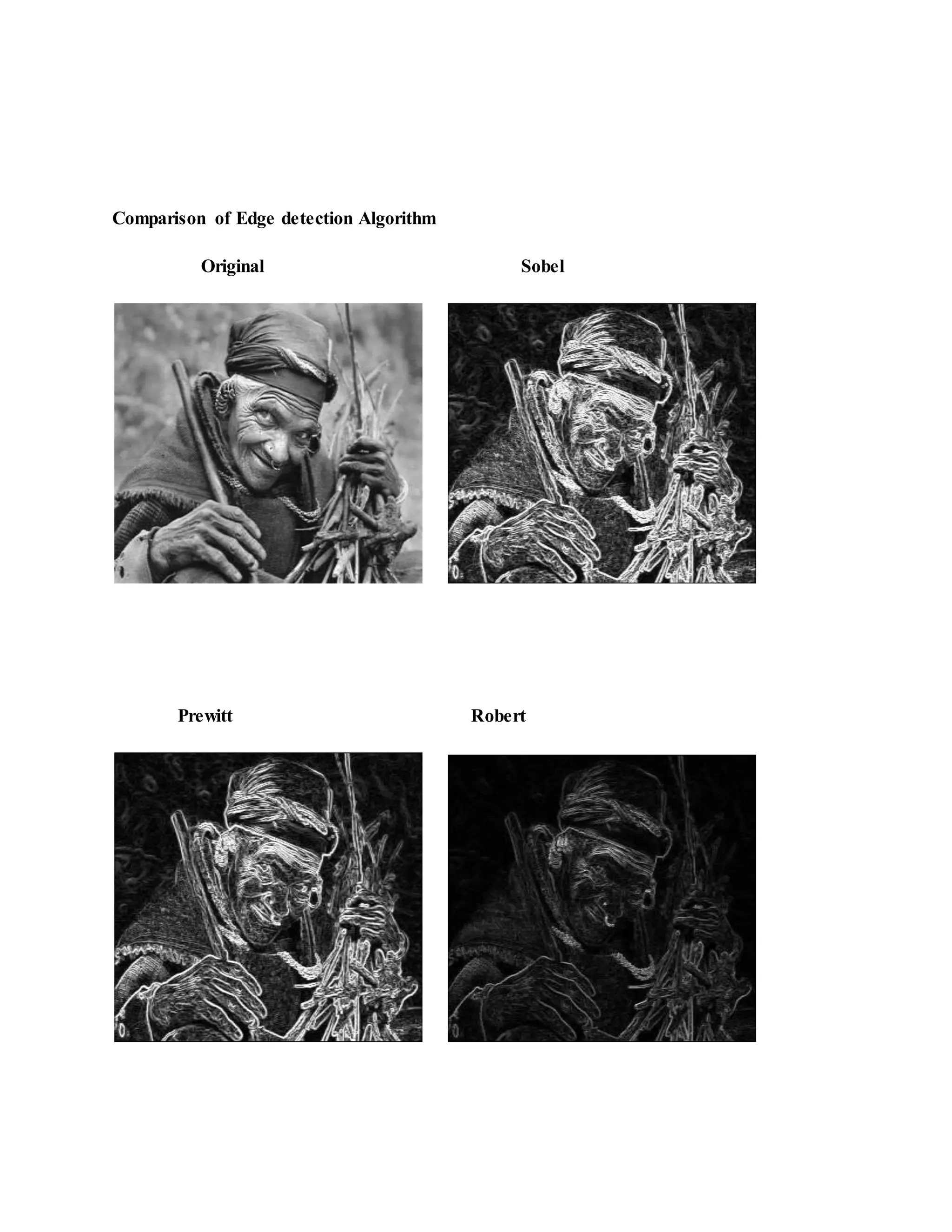
4.4 COMPARISON OF VARIOUS EDGE DETECTIONALGORITHMS
Edge detection of all four types was performed on Figure 4.11 Canny yielded the best results.
This was expected as Canny edge detection accounts for regions in an image[35]. Canny yields
thin lines for its edges by using non-maximal suppression. Canny also utilizes hysteresis when
thresholding.

15. Figure 4.11 Image used for edge detection analysis (wheel.gif)
Figure 4.12: Results of edge detection on Figure 4.11. Notice Canny had the best results.

16. Motion blur was applied to Figure 4.13. Then, the edge detection methods previously used were
utilized again on this new image to study their affects in blurry image environments [34]. No
method appeared to be useful for real world applications. However, Canny produced the best the
results out of the set.
Figure 4.13 Result of edge detection

17. Comparison of Edge detection Algorithm
Original Sobel
Prewitt Robert

18. Laplacian Laplacian of Gaussian
Performance of Edge Detection Algorithms
 Gradient-based algorithms such as the Prewitt filter have a major drawback of being very
sensitive to noise. The size of the kernel filter and coefficients are fixed and cannot be
adapted to a given image. An adaptive edge-detection algorithm is necessary to provide a
robust solution that is adaptable to the varying noise levels. Gradient-based algorithms such
as the Prewitt filter have a major drawback of being very sensitive to noise. The size of the
kernel filter and coefficients are fixed and cannot be adapted to a given image. An adaptive
edge-detection algorithm is necessary to provide a robust solution that is adaptable to the
varying noise levels of these images to help distinguish valid image contents from visual
artifacts introduced by noise[34,35].
 The performance of the Canny algorithm depends heavily on the adjustable parameters, σ,
which is the standard deviation for the Gaussian filter, and the threshold values, ‘T1’ and

19. ‘T2’. σ also controls the size of the Gaussian filter. The bigger the value for σ, the larger the
size of the Gaussian filter becomes. This implies more blurring, necessary for noisy images,
as well as detecting larger edges. As expected, however, the larger the scale of the Gaussian,
the less accurate is the localization of the edge. Smaller values of σ imply a smaller
Gaussian filter which limits the amount of blurring, maintaining finer edges in the image.
The user can tailor the algorithm by adjusting these parameters to adapt to different
environments.
 Canny’s edge detection algorithm is computationally more expensive compared to Sobel,
Prewitt and Robert’s operator. However, the Canny’s edge detection algorithm performs
better than all these operators under almost all scenarios[27,35].
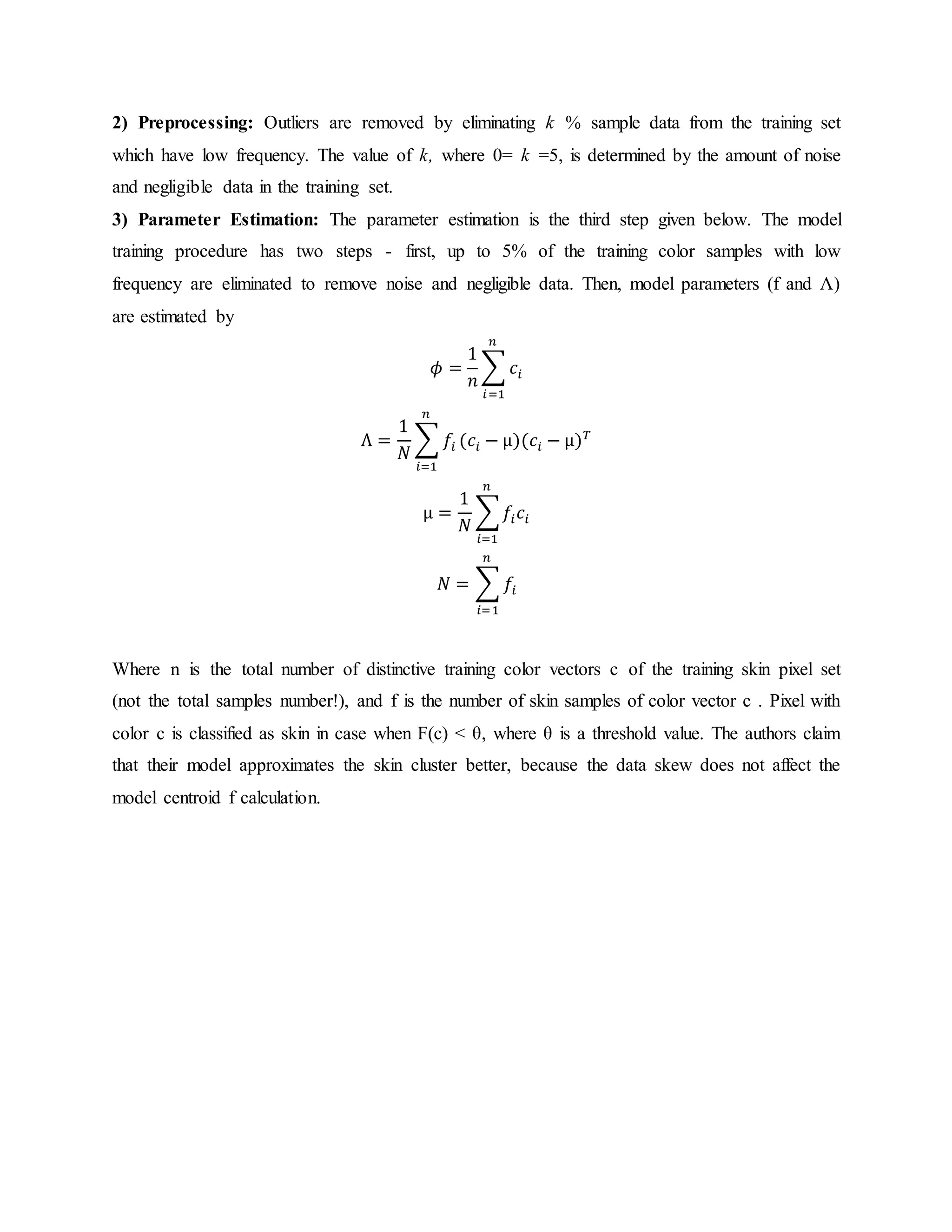
4.5 ELLIPTICAL BOUNDARYMODEL
There is a new statistical color model for skin detection, called an elliptical boundary model.
This model is trained from a set of training data in two steps, preprocessing and parameter
estimation. In preprocessing step we remove outliers so that the trained model reflects the main
density of the underlying data set.
By examining skin and non-skin distributions in several color spaces Lee and Yoo [36] have
concluded that skin color cluster, being approximately elliptic in shape is not well enough
approximated by the single Gaussian model. Due to asymmetry of the skin cluster with respect to
its density peak, usage of the symmetric Gaussian model leads to high false positives rate. They
propose an alternative they call an ”elliptical boundary model” which is equally fast and simple
in training and evaluation as the single Gaussian model and gives superior detection results on
the Compaq database [37] compared both to single and mixture of Gaussians . The elliptical
boundary model is defined as:
Φ( 𝑐) = (𝑐 − ∅) 𝑇
Λ−1
(𝑐 − ∅)
This model is trained from a set of training data in two steps, preprocessing and parameter
estimation. In preprocessing step we remove outliers so that the trained model reflects the main
density of the underlying data set. In parameter estimation step we estimate model parameters
from the preprocessed data set.
1) Training Data Set: Initially training data set consists of skin chrominance samples.

20. 2) Preprocessing: Outliers are removed by eliminating k % sample data from the training set
which have low frequency. The value of k, where 0= k =5, is determined by the amount of noise
and negligible data in the training set.
3) Parameter Estimation: The parameter estimation is the third step given below. The model
training procedure has two steps - first, up to 5% of the training color samples with low
frequency are eliminated to remove noise and negligible data. Then, model parameters (f and Λ)
are estimated by
𝜙 =
1
𝑛
∑ 𝑐𝑖
𝑛
𝑖=1
Λ =
1
𝑁
∑ 𝑓𝑖
𝑛
𝑖=1
(𝑐𝑖 − μ)(𝑐𝑖 − μ) 𝑇
μ =
1
𝑁
∑ 𝑓𝑖 𝑐𝑖
𝑛
𝑖=1
𝑁 = ∑ 𝑓𝑖
𝑛
𝑖=1
Where n is the total number of distinctive training color vectors c of the training skin pixel set
(not the total samples number!), and f is the number of skin samples of color vector c . Pixel with
color c is classified as skin in case when F(c) < θ, where θ is a threshold value. The authors claim
that their model approximates the skin cluster better, because the data skew does not affect the
model centroid f calculation.