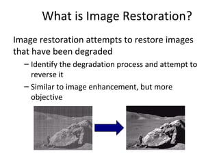
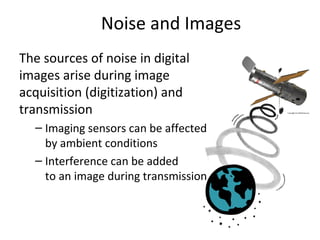
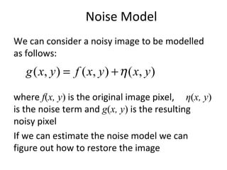
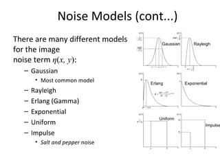
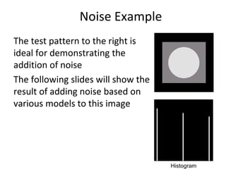
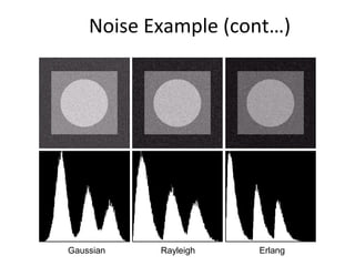
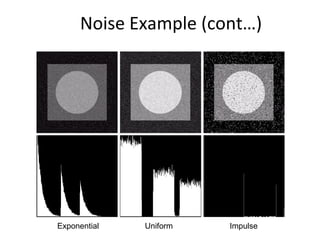
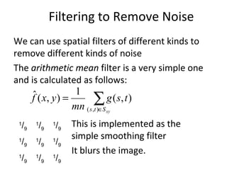
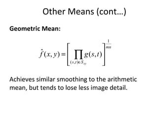
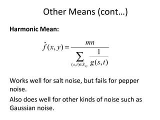
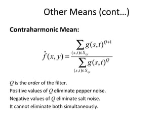
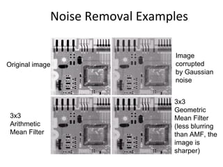
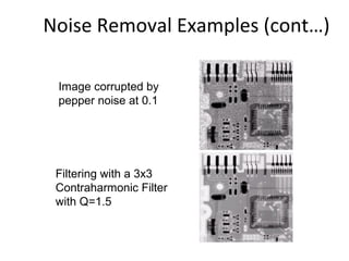
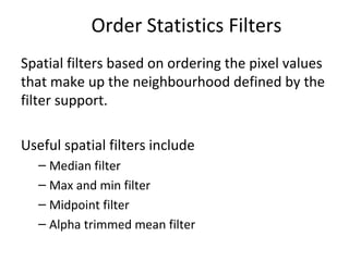
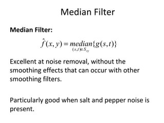
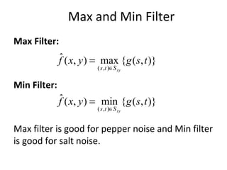
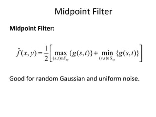
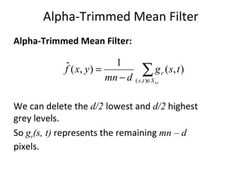
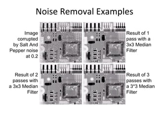
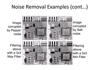
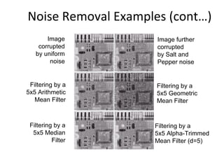
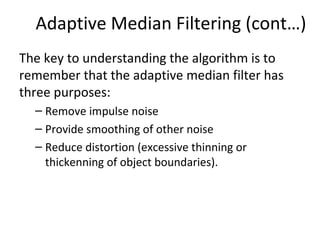
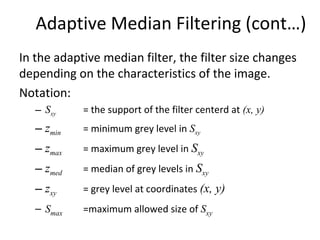
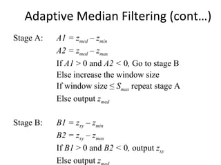
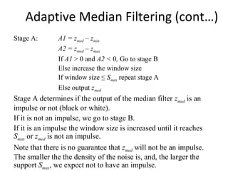
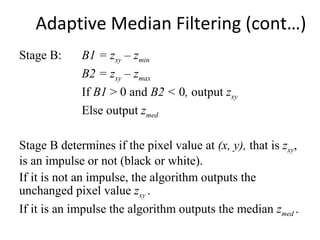
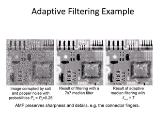
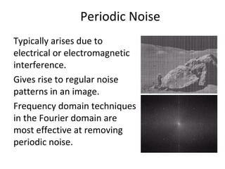
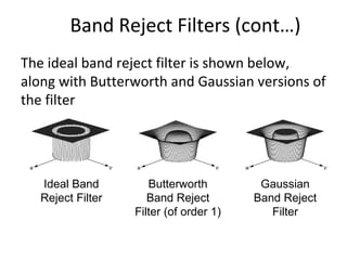
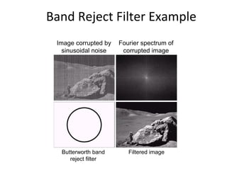
Quality defects in TMT Bars, Possible causes and Potential Solutions.
Chapter 5
1. Image Restoration and Reconstruction
(Noise Removal)
Subject: FIP (181102)
Prof. Asodariya Bhavesh
ECD,SSASIT, Surat
2. Image Restoration and
Reconstruction
Things which we see are not by themselves what we
see…
It remains completely unknown to us what the objects
may be by themselves and apart from the receptivity of
our senses. We know nothing but our manner of
perceiving them.
Immanuel Kant
3. Contents
In this lecture we will look at image restoration
techniques used for noise removal
– What is image restoration?
– Noise and images
– Noise models
– Noise removal using spatial domain filtering
– Noise removal using frequency domain filtering
4. What is Image Restoration?
Image restoration attempts to restore images
that have been degraded
– Identify the degradation process and attempt to
reverse it
– Similar to image enhancement, but more
objective
5. Noise and Images
The sources of noise in digital
images arise during image
acquisition (digitization) and
transmission
– Imaging sensors can be affected
by ambient conditions
– Interference can be added
to an image during transmission
6. Noise Model
We can consider a noisy image to be modelled
as follows:
where f(x, y) is the original image pixel, η(x, y)
is the noise term and g(x, y) is the resulting
noisy pixel
If we can estimate the noise model we can
figure out how to restore the image
),(),(),( yxyxfyxg η+=
7. Noise Models (cont...)
Gaussian Rayleigh
Erlang Exponential
Uniform
Impulse
There are many different models
for the image
noise term η(x, y):
– Gaussian
• Most common model
– Rayleigh
– Erlang (Gamma)
– Exponential
– Uniform
– Impulse
• Salt and pepper noise
8. Noise Example
The test pattern to the right is
ideal for demonstrating the
addition of noise
The following slides will show the
result of adding noise based on
various models to this image
Histogram to go here
Histogram
11. We can use spatial filters of different kinds to
remove different kinds of noise
The arithmetic mean filter is a very simple one
and is calculated as follows:
This is implemented as the
simple smoothing filter
It blurs the image.
∑∈
=
xySts
tsg
mn
yxf
),(
),(
1
),(ˆ
1
/9
1
/9
1
/9
1
/9
1
/9
1
/9
1
/9
1
/9
1
/9
Filtering to Remove Noise
12. Other Means
There are different kinds of mean filters all of
which exhibit slightly different behaviour:
– Geometric Mean
– Harmonic Mean
– Contraharmonic Mean
13. Other Means (cont…)
Geometric Mean:
Achieves similar smoothing to the arithmetic
mean, but tends to lose less image detail.
mn
Sts xy
tsgyxf
1
),(
),(),(ˆ
= ∏∈
14. Harmonic Mean:
Works well for salt noise, but fails for pepper
noise.
Also does well for other kinds of noise such as
Gaussian noise.
∑∈
=
xySts tsg
mn
yxf
),( ),(
1
),(ˆ
Other Means (cont…)
15. Other Means (cont…)
Contraharmonic Mean:
Q is the order of the filter.
Positive values of Q eliminate pepper noise.
Negative values of Q eliminate salt noise.
It cannot eliminate both simultaneously.
∑
∑
∈
∈
+
=
xy
xy
Sts
Q
Sts
Q
tsg
tsg
yxf
),(
),(
1
),(
),(
),(ˆ
16. Noise Removal Examples
Original image
Image
corrupted
by Gaussian
noise
3x3
Geometric
Mean Filter
(less blurring
than AMF, the
image is
sharper)
3x3
Arithmetic
Mean Filter
17. Noise Removal Examples (cont…)
Image corrupted by
pepper noise at 0.1
Filtering with a 3x3
Contraharmonic Filter
with Q=1.5
18. Noise Removal Examples (cont…)
Image corrupted by
salt noise at 0.1
Filtering with a 3x3
Contraharmonic Filter
with Q=-1.5
19. Contraharmonic Filter: Here Be Dragons
Choosing the wrong value for Q when using the
contraharmonic filter can have drastic results
Pepper noise filtered by
a 3x3 CF with Q=-1.5
Salt noise filtered by a
3x3 CF with Q=1.5
20. Order Statistics Filters
Spatial filters based on ordering the pixel values
that make up the neighbourhood defined by the
filter support.
Useful spatial filters include
– Median filter
– Max and min filter
– Midpoint filter
– Alpha trimmed mean filter
21. Median Filter
Median Filter:
Excellent at noise removal, without the
smoothing effects that can occur with other
smoothing filters.
Particularly good when salt and pepper noise is
present.
)},({),(ˆ
),(
tsgmedianyxf
xySts ∈
=
22. Max and Min Filter
Max Filter:
Min Filter:
Max filter is good for pepper noise and Min filter
is good for salt noise.
)},({max),(ˆ
),(
tsgyxf
xySts ∈
=
)},({min),(ˆ
),(
tsgyxf
xySts ∈
=
24. Alpha-Trimmed Mean Filter
Alpha-Trimmed Mean Filter:
We can delete the d/2 lowest and d/2 highest
grey levels.
So gr(s, t) represents the remaining mn – d
pixels.
∑∈−
=
xySts
r tsg
dmn
yxf
),(
),(
1
),(ˆ
25. Noise Removal Examples
Image
corrupted
by Salt And
Pepper noise
at 0.2
Result of 1
pass with a
3x3 Median
Filter
Result of 2
passes with
a 3x3 Median
Filter
Result of 3
passes with
a 3*3 Median
Filter
26. Noise Removal Examples (cont…)
Image
corrupted
by Pepper
noise
Image
corrupted
by Salt
noise
Filtering
above
with a 3x3
Min Filter
Filtering
above
with a 3x3
Max Filter
27. Noise Removal Examples (cont…)
Image
corrupted
by uniform
noise
Image further
corrupted
by Salt and
Pepper noise
Filtering by a
5x5 Arithmetic
Mean Filter
Filtering by a
5x5 Median
Filter
Filtering by a
5x5 Geometric
Mean Filter
Filtering by a
5x5 Alpha-Trimmed
Mean Filter (d=5)
28. Adaptive Filters
The filters discussed so far are applied to an
entire image without any regard for how image
characteristics vary from one point to another.
The behaviour of adaptive filters changes
depending on the characteristics of the image
inside the filter region.
We will take a look at the adaptive median
filter.
29. Adaptive Median Filtering
The median filter performs relatively well on
impulse noise as long as the spatial density of
the impulse noise is not large.
The adaptive median filter can handle much
more spatially dense impulse noise, and also
performs some smoothing for non-impulse
noise.
30. Adaptive Median Filtering (cont…)
The key to understanding the algorithm is to
remember that the adaptive median filter has
three purposes:
– Remove impulse noise
– Provide smoothing of other noise
– Reduce distortion (excessive thinning or
thickenning of object boundaries).
31. Adaptive Median Filtering (cont…)
In the adaptive median filter, the filter size changes
depending on the characteristics of the image.
Notation:
– Sxy = the support of the filter centerd at (x, y)
– zmin = minimum grey level in Sxy
– zmax = maximum grey level in Sxy
– zmed = median of grey levels in Sxy
– zxy = grey level at coordinates (x, y)
– Smax =maximum allowed size of Sxy
32. Adaptive Median Filtering (cont…)
Stage A: A1 = zmed – zmin
A2 = zmed – zmax
If A1 > 0 and A2 < 0, Go to stage B
Else increase the window size
If window size ≤ Smax repeat stage A
Else output zmed
Stage B: B1 = zxy – zmin
B2 = zxy – zmax
If B1 > 0 and B2 < 0, output zxy
Else output z
33. Adaptive Median Filtering (cont…)
Stage A: A1 = zmed – zmin
A2 = zmed – zmax
If A1 > 0 and A2 < 0, Go to stage B
Else increase the window size
If window size ≤ Smax repeat stage A
Else output zmed
Stage A determines if the output of the median filter zmed is an
impulse or not (black or white).
If it is not an impulse, we go to stage B.
If it is an impulse the window size is increased until it reaches
Smax or zmed is not an impulse.
Note that there is no guarantee that zmed will not be an impulse.
The smaller the the density of the noise is, and, the larger the
support Smax, we expect not to have an impulse.
34. Adaptive Median Filtering (cont…)
Stage B: B1 = zxy – zmin
B2 = zxy – zmax
If B1 > 0 and B2 < 0, output zxy
Else output zmed
Stage B determines if the pixel value at (x, y), that is zxy,
is an impulse or not (black or white).
If it is not an impulse, the algorithm outputs the
unchanged pixel value zxy .
If it is an impulse the algorithm outputs the median zmed .
35. Adaptive Filtering Example
Image corrupted by salt
and pepper noise with
probabilities Pa = Pb=0.25
Result of filtering with a
7x7 median filter
Result of adaptive
median filtering with
Smax = 7
AMF preserves sharpness and details, e.g. the connector fingers.
36. Periodic Noise
Typically arises due to
electrical or electromagnetic
interference.
Gives rise to regular noise
patterns in an image.
Frequency domain techniques
in the Fourier domain are
most effective at removing
periodic noise.
37. Band Reject Filters
Removing periodic noise form an image involves
removing a particular range of frequencies from
that image.
Band reject filters can be used for this purpose
An ideal band reject filter is given as follows:
+>
+≤≤−
−<
=
2
),(1
2
),(
2
0
2
),(1
),(
0
00
0
W
DvuDif
W
DvuD
W
Dif
W
DvuDif
vuH
38. Band Reject Filters (cont…)
The ideal band reject filter is shown below,
along with Butterworth and Gaussian versions of
the filter
Ideal Band
Reject Filter
Butterworth
Band Reject
Filter (of order 1)
Gaussian
Band Reject
Filter
39. Band Reject Filter Example
Image corrupted by
sinusoidal noise
Fourier spectrum of
corrupted image
Butterworth band
reject filter
Filtered image