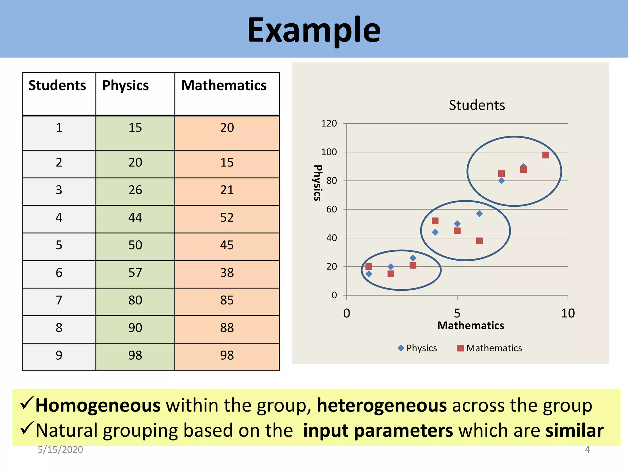
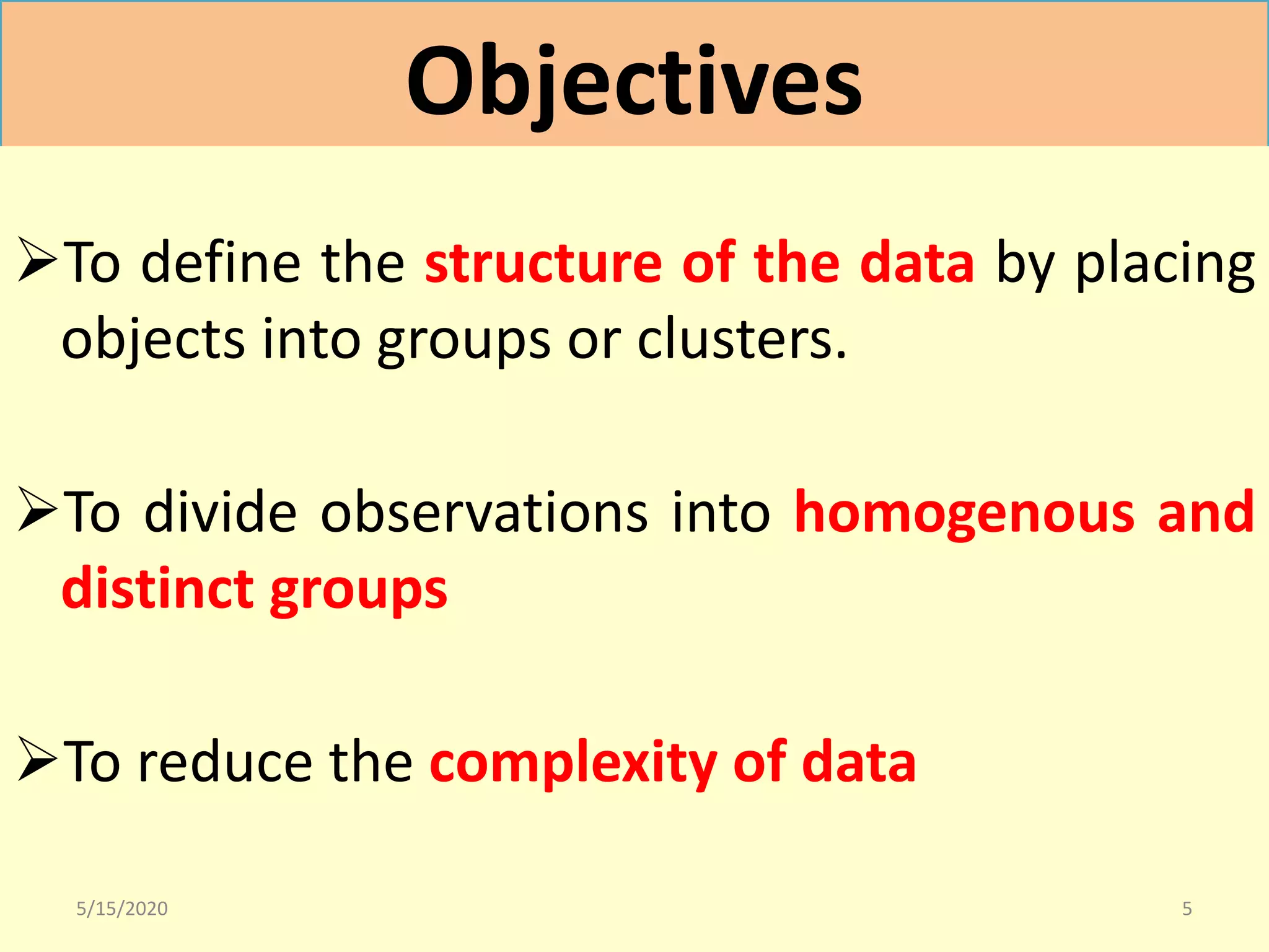
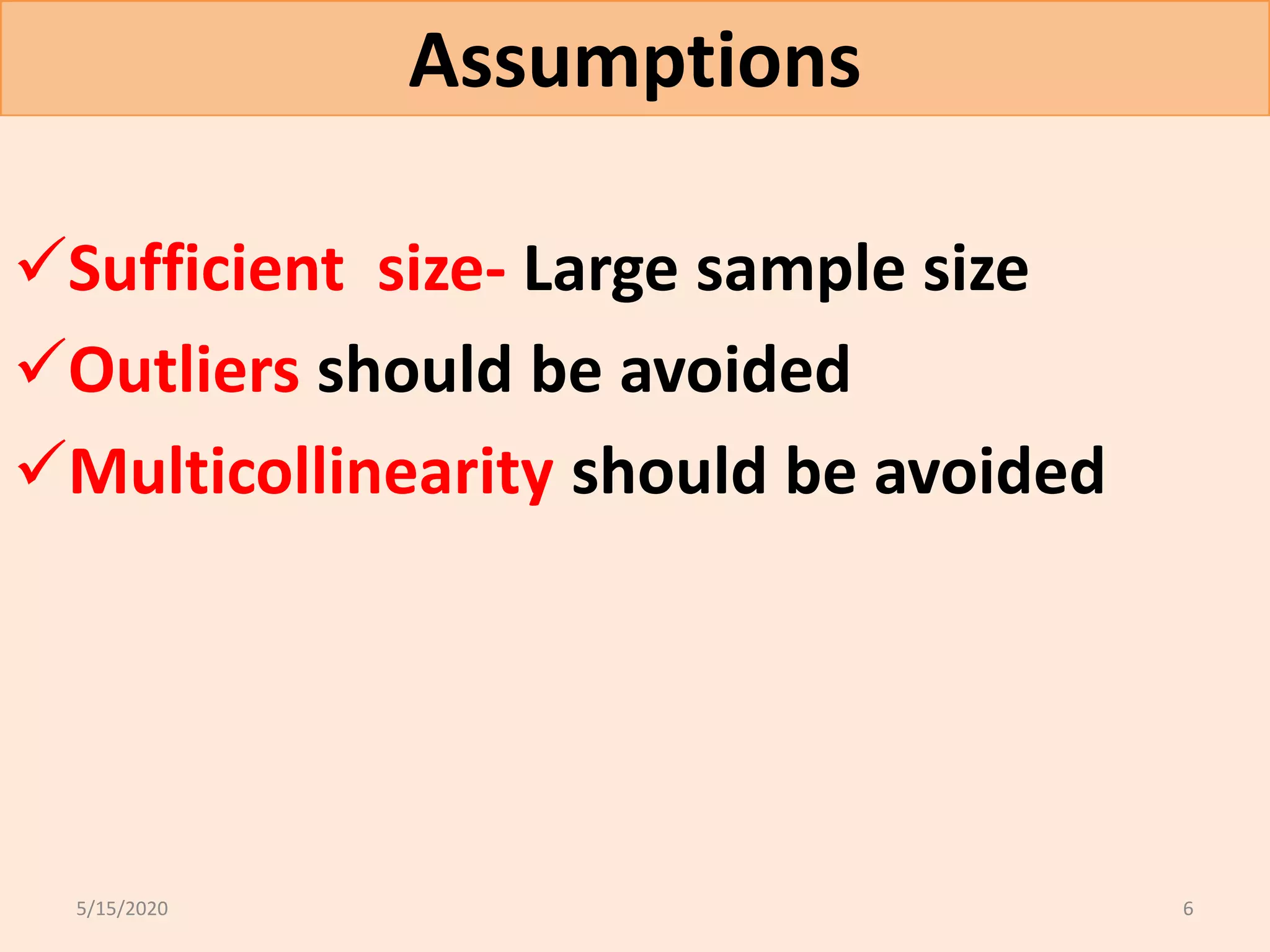
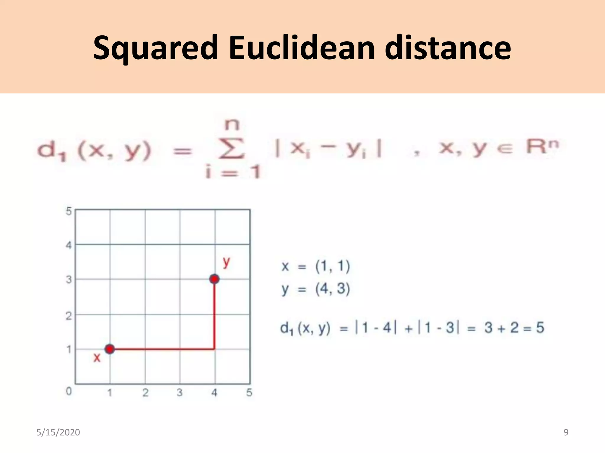
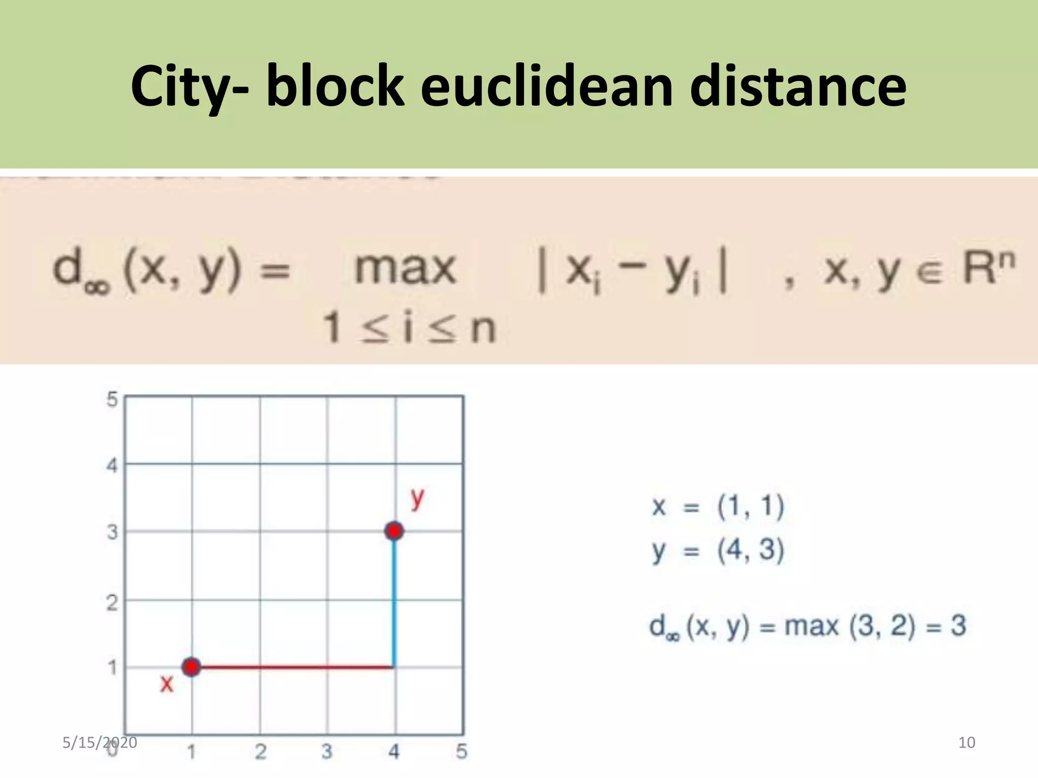
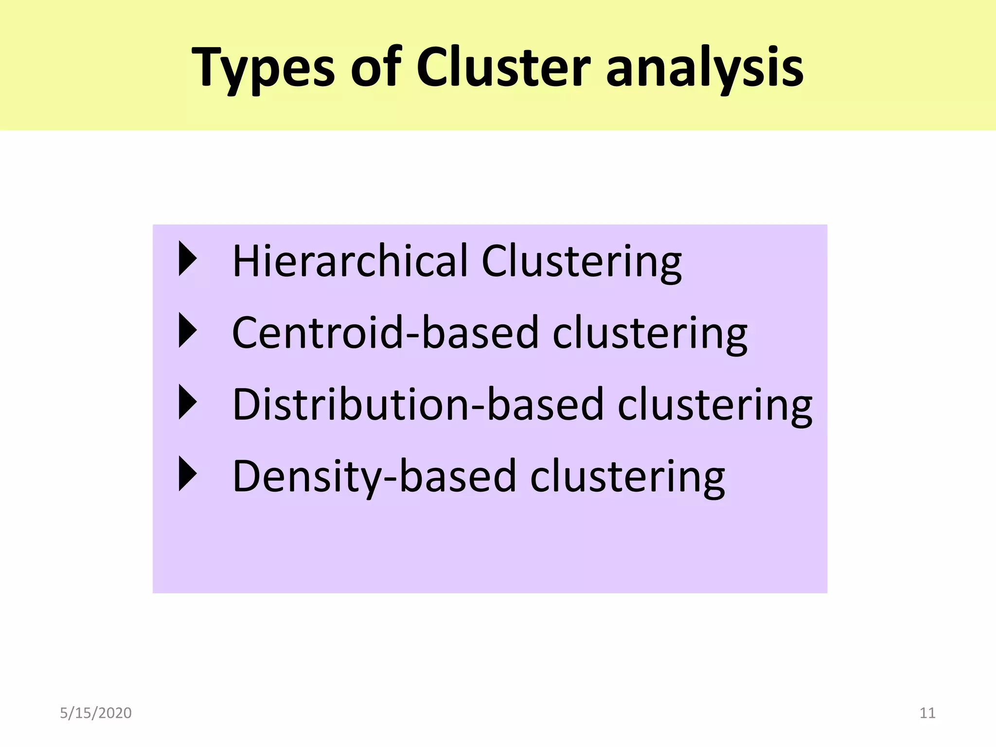
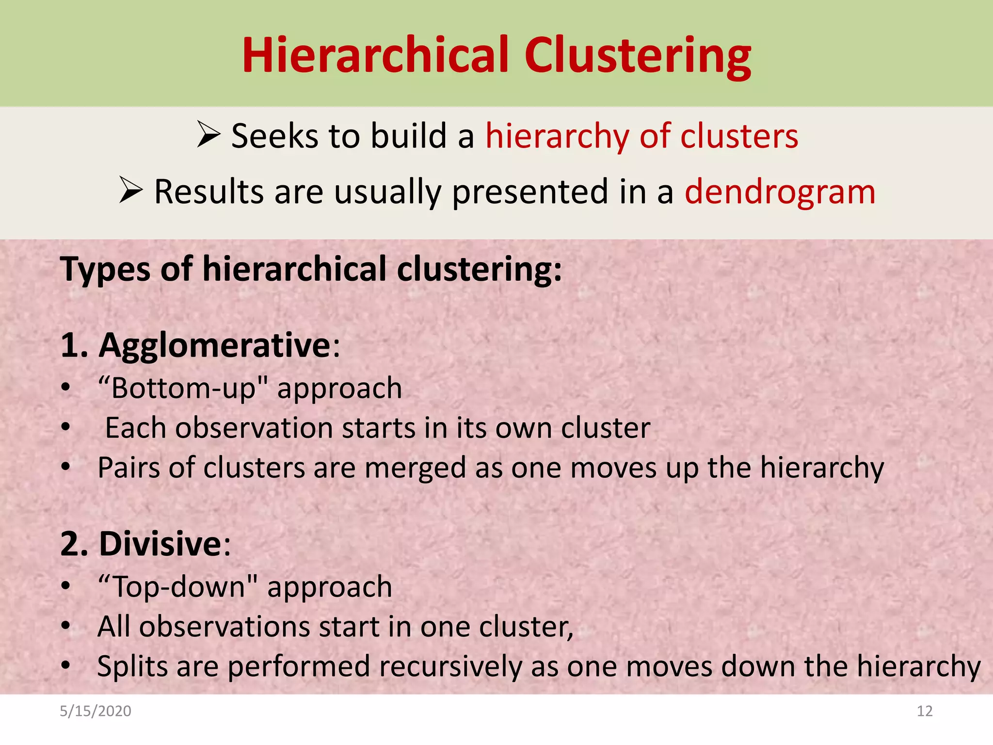
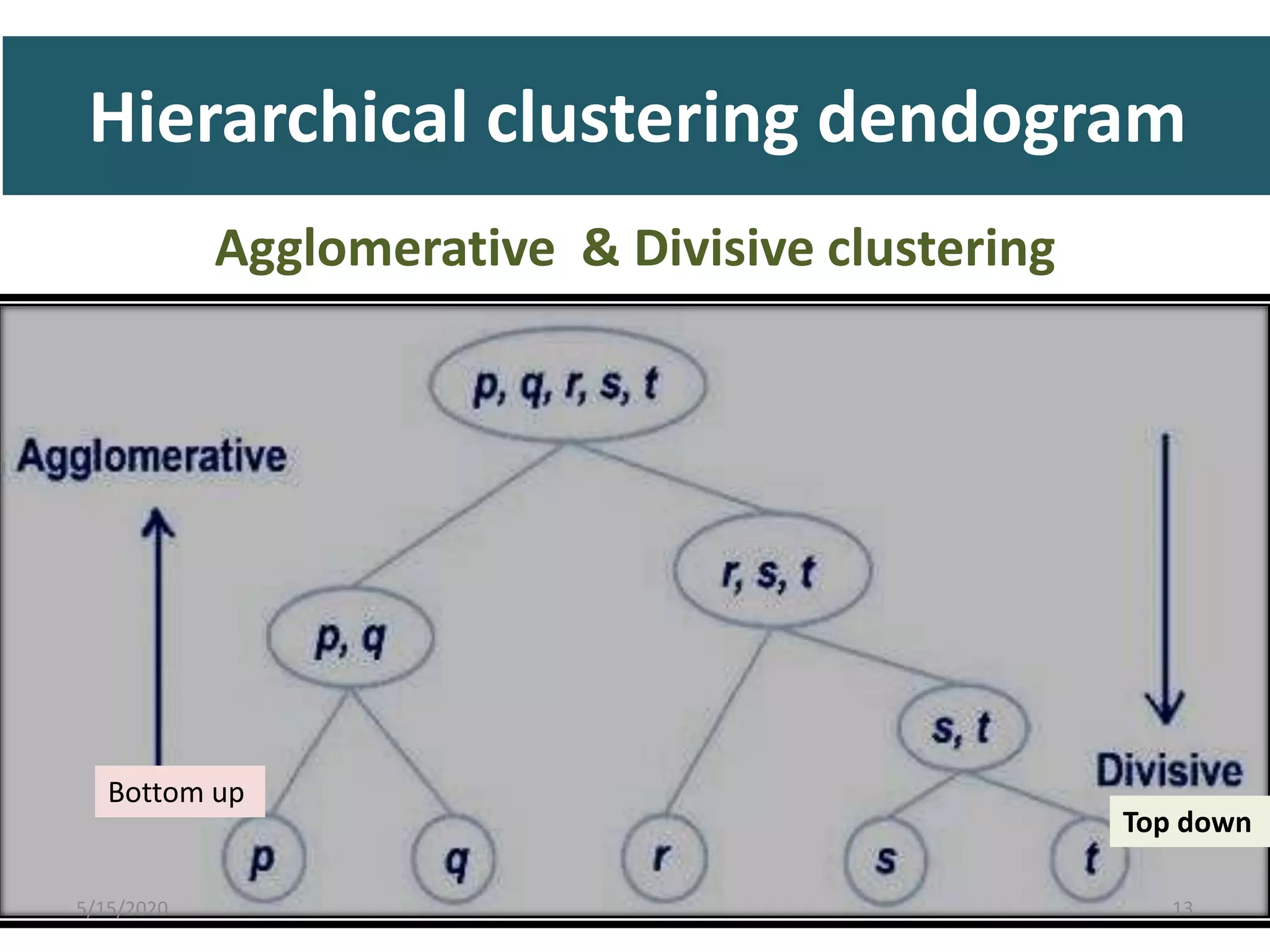
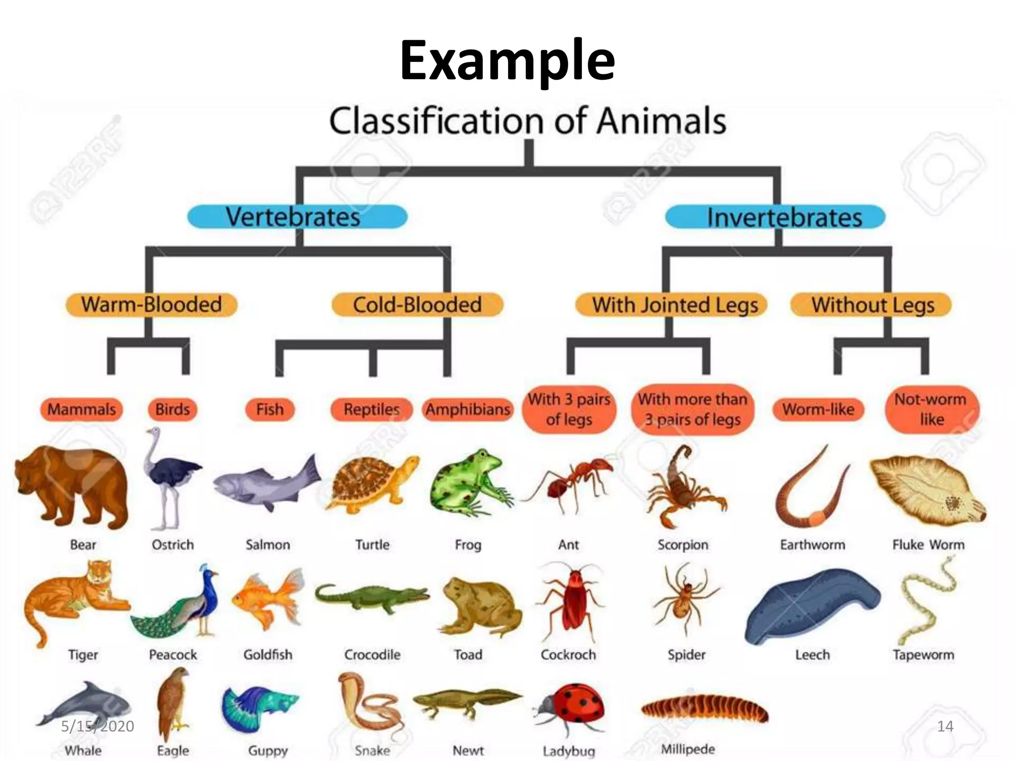
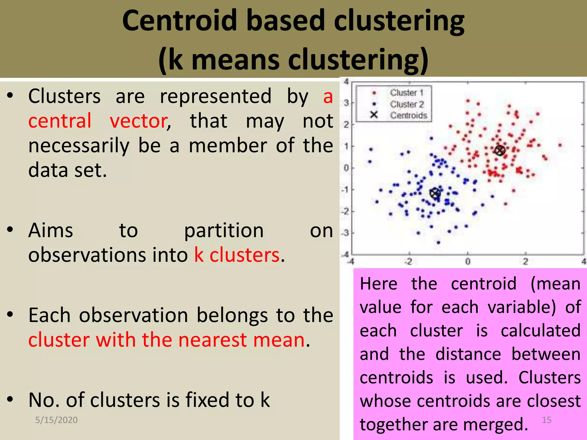
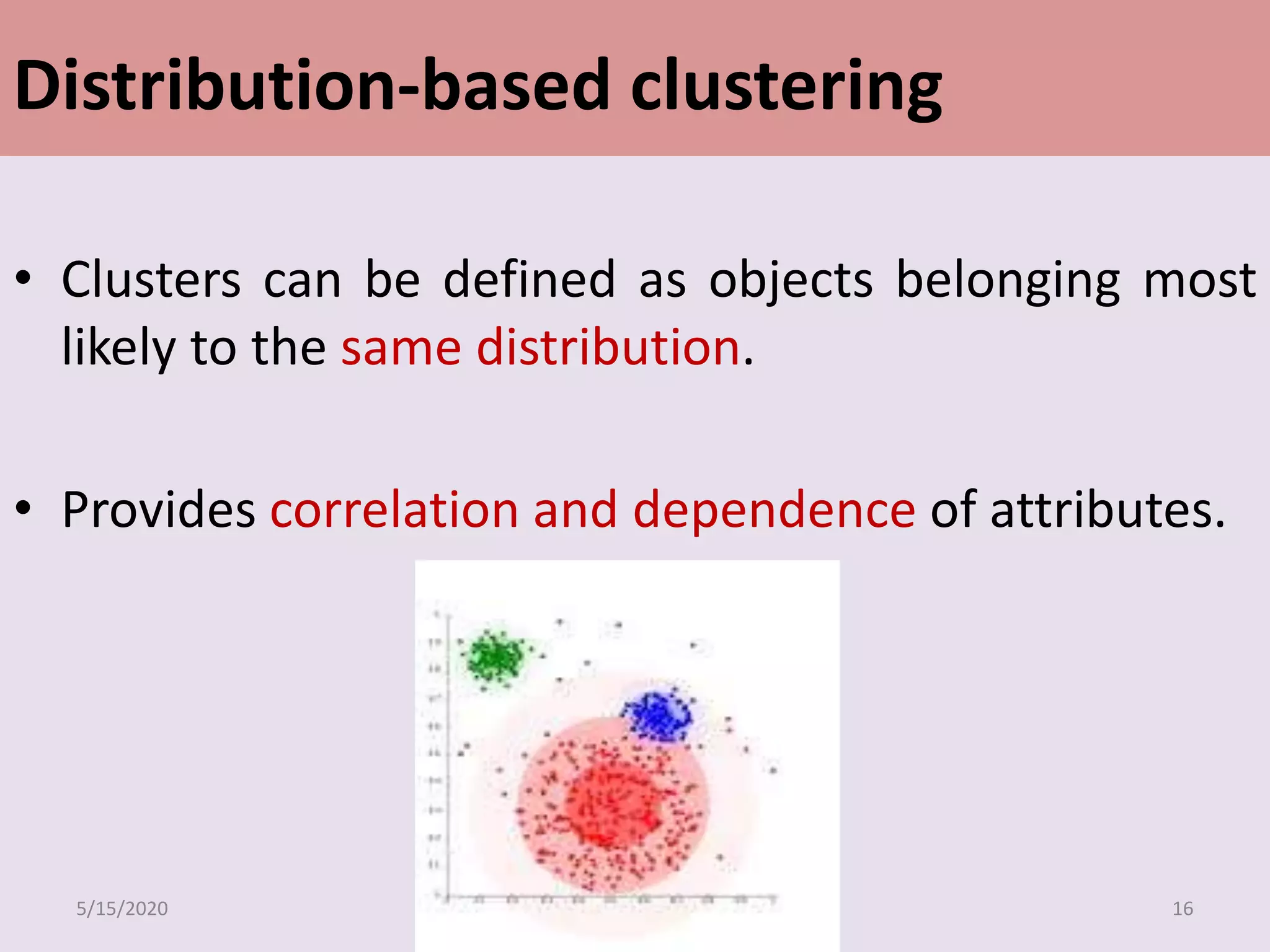
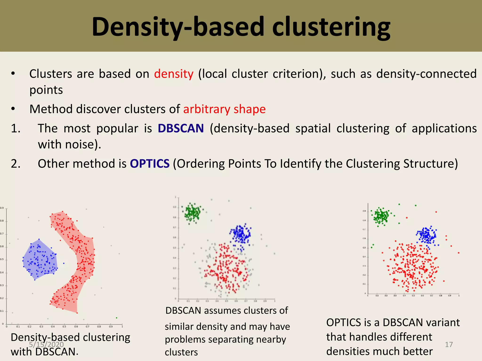
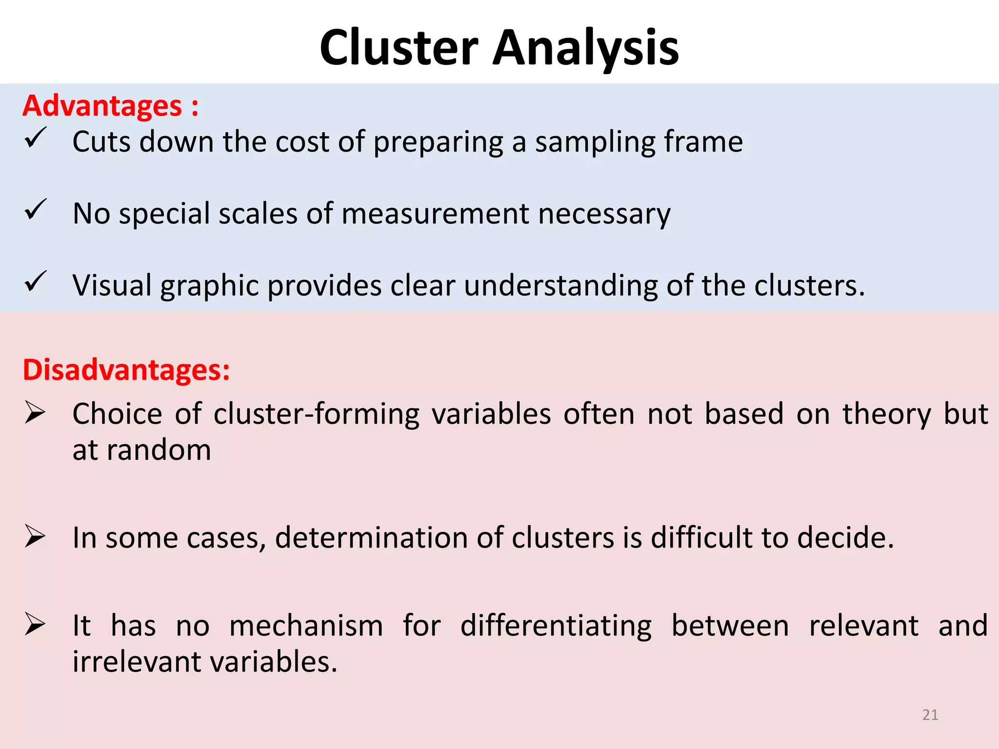
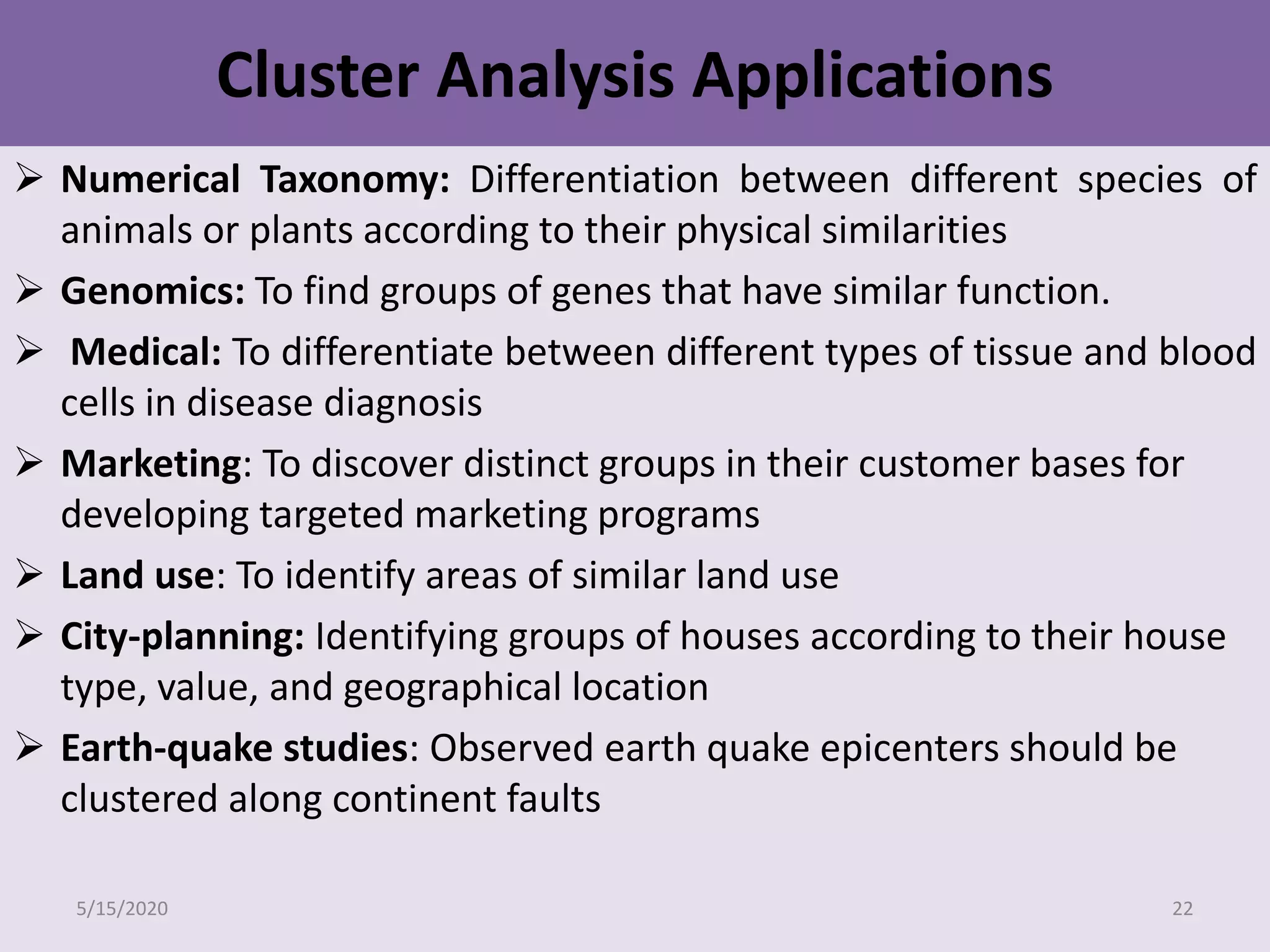
Suchismita Prusty FEX-PA9-03,
ICAR- Central Institute Of Fisheries Education
5/15/2020 1
Introduction
It is a multivariate statistical technique designed to
group the objects based on the homogeneity of
characteristics or attributes.
It provides sensible and informative classification
of an initially unclassified set of data
It saves lot of resource in terms of time and money
5/15/2020 2
 This analysis generates several groups of data sets
which are similar.
 Similar means homogeneous within the group and
as much as possible heterogeneous to other
groups
 Segregation is done based on more than two
variables.
What cluster analysis does?
5/15/2020 3
Example
Students Physics Mathematics
1 15 20
2 20 15
3 26 21
4 44 52
5 50 45
6 57 38
7 80 85
8 90 88
9 98 98
0
20
40
60
80
100
120
0 5 10
Physics Mathematics
Physics
Mathematics
Students
Homogeneous within the group, heterogeneous across the group
Natural grouping based on the input parameters which are similar
5/15/2020 4
Objectives
To define the structure of the data by placing
objects into groups or clusters.
To divide observations into homogenous and
distinct groups
To reduce the complexity of data
5/15/2020 5
Assumptions
Sufficient size- Large sample size
Outliers should be avoided
Multicollinearity should be avoided
5/15/2020 6
Measuring Similarity
Similarity :- degree of correspondence among objects across
all of the characteristics
Distance Measures
 Euclidean distance :-The most commonly recognized to as
straight- line distance
 Squared Euclidean distance:-The sum of the squared
differences without taking the square root
 City- block euclidean distance:-Uses the sum of the variables
absolute differences5/15/2020 7
Euclidean distance
5/15/2020 8
Squared Euclidean distance
5/15/2020 9
City- block euclidean distance
5/15/2020 10
Types of Cluster analysis
 Hierarchical Clustering
 Centroid-based clustering
 Distribution-based clustering
 Density-based clustering
5/15/2020 11
Hierarchical Clustering
 Seeks to build a hierarchy of clusters
 Results are usually presented in a dendrogram
Types of hierarchical clustering:
1. Agglomerative:
• “Bottom-up" approach
• Each observation starts in its own cluster
• Pairs of clusters are merged as one moves up the hierarchy
2. Divisive:
• “Top-down" approach
• All observations start in one cluster,
• Splits are performed recursively as one moves down the hierarchy
5/15/2020 12
Hierarchical clustering dendogram
Agglomerative & Divisive clustering
Bottom up
Top down
5/15/2020 13
Example
5/15/2020 14
Centroid based clustering
(k means clustering)
• Clusters are represented by a
central vector, that may not
necessarily be a member of the
data set.
• Aims to partition on
observations into k clusters.
• Each observation belongs to the
cluster with the nearest mean.
• No. of clusters is fixed to k
Here the centroid (mean
value for each variable) of
each cluster is calculated
and the distance between
centroids is used. Clusters
whose centroids are closest
together are merged.5/15/2020 15
Distribution-based clustering
• Clusters can be defined as objects belonging most
likely to the same distribution.
• Provides correlation and dependence of attributes.
5/15/2020 16
Density-based clustering
• Clusters are based on density (local cluster criterion), such as density-connected
points
• Method discover clusters of arbitrary shape
1. The most popular is DBSCAN (density-based spatial clustering of applications
with noise).
2. Other method is OPTICS (Ordering Points To Identify the Clustering Structure)
Density-based clustering
with DBSCAN.
DBSCAN assumes clusters of
similar density and may have
problems separating nearby
clusters
OPTICS is a DBSCAN variant
that handles different
densities much better
5/15/2020 17
1.One phase clustering- Forming the clusters from
the given data set, resulting in a new variable that
identifies cluster members among the cases
2. Two Phase Cluster- Description of clusters by re-
crossing with the data
EXAMPLE
5/15/2020 18
Survey of marine fishing vessels
Mechanised
Motorised
Traditional
One phase cluster
Forming of clusters by the
chosen data set
5/15/2020 19
Mechanised
Registered
Non-
registered
>10 years
old
<10years
old
Two phase cluster
Third phase cluster
5/15/2020 20
Disadvantages:
 Choice of cluster-forming variables often not based on theory but
at random
 In some cases, determination of clusters is difficult to decide.
 It has no mechanism for differentiating between relevant and
irrelevant variables.
Cluster Analysis
Advantages :
 Cuts down the cost of preparing a sampling frame
 No special scales of measurement necessary
 Visual graphic provides clear understanding of the clusters.
21
Cluster Analysis Applications
 Numerical Taxonomy: Differentiation between different species of
animals or plants according to their physical similarities
 Genomics: To find groups of genes that have similar function.
 Medical: To differentiate between different types of tissue and blood
cells in disease diagnosis
 Marketing: To discover distinct groups in their customer bases for
developing targeted marketing programs
 Land use: To identify areas of similar land use
 City-planning: Identifying groups of houses according to their house
type, value, and geographical location
 Earth-quake studies: Observed earth quake epicenters should be
clustered along continent faults
5/15/2020 22
Hierarchial Cluster analysis in SPSS
• Let’s take a very basic example
• Imagine we wanted to look at clusters of cases referred for psychiatric
treatment
• We measured each subject on 4 questionnaires:
1. Spielberger Trait Anxiety Inventory (STAI)
2. Beck Depression Inventory (BDI)
3. Intrusive Thoughts and Rumination (IT)
4. Impulsive Thoughts and Actions (Impulse)
• Rationale - People with the same disorder should report a similar
pattern(DSM) of scores across the measures
Data
DSM STAI BDI IT IMPULSE
GAD 74 30 20 10
Depression 50 70 23 5
OCD 70 5 58 29
GAD 76 35 23 12
OCD 68 23 66 37
OCD 62 8 59 39
GAD 71 35 27 17
OCD 67 12 65 35
Depression 35 60 15 8
Depression 33 58 11 16
GAD 80 36 30 16
Depression 30 62 9 13
GAD 65 38 17 10
OCD 78 15 70 40
Depression 40 55 10 2
Running the analysis
This dialogue box is obtained using the menu path Analyze-
>Classify->Hierarchical Cluster
• Select the 4 diagnostic questionnaires from the left and drag them to
the variable box.
• The variable DSM is included in the data editor to demonstrate what
the output from a cluster analysis means
• If you click on Statistics in the main dialog box then another dialog
box appears
• By default, SPSS will simply merge all cases into a single cluster and it
is down to the researcher to inspect the output to determine
substantive sub-clusters.
• However, if you have a hypothesis about how many clusters should
emerge, then you can tell SPSS to create a set number of clusters, or
to create a number of clusters within a range.
• For this example, leave the default options as they are and proceed
back to the main dialog box by clicking Continue.
• Click on Method … to access the dialog box
• The most useful for interpretation purposes is the dendrogram.
• It shows us the forks (or links) between cases and its structure gives
us clues as to which cases form coherent clusters. click on Continue.
• Once back in the main dialog box, you can select the save
dialog box by clicking Save ….
• This dialog box allows us to save a new variable into the data
editor that contains a coding value representing membership
to a cluster.
• We could select Single solution and then type 3 in the blank
space.
Output
• The main part of the output from SPSS is the dendrogram
(although ironically this graph appears only if a special
option is selected). The dendrogram for the diagnosis data
is presented in output.
• For these data, the fork first splits to separate cases 1, 4, 7, 11, 13, 10, 12, 9, 15, & 2
from cases 5, 14, 6, 8, & 3.
• If you look at the DSM-IV classification for these subjects, this first separation has
divided up GAD and Depression from OCD. This is likely to have occurred because
both GAD and Depression patients have low scores on intrusive thoughts and
impulsive thoughts and actions whereas those with OCD score highly on both
measures.
• The second major division is to split one branch of this first fork into two further
clusters. This division separates cases 1, 4, 7, 11 & 13 from 10, 12, 9, 15, &
2.Looking at the DSM classification this second split has separated GAD from
Depression.
• In short, the final analysis has revealed 3 major clusters, which seem to be related
to the classifications arising from DSM. As such, we can argue that using the STAI,
BDI, IT and Impulse as diagnostic measures is an accurate way to classify these
three groups of patients (and possibly less time consuming than a full DSM-IV
diagnosis).
• In reality there is a lot subjectivity involved in deciding
which clusters are substantive.
• Having eyeballed the dendrogram to decide how many
clusters are present it is possible to re-run the analysis
asking SPSS to save a new variable in which cluster codes
are assigned to cases (with the researcher specifying the
number of clusters in the data).
• Although this example is very simplistic it shows you how
useful cluster analysis can be in developing and validating
diagnostic tools, or in establishing natural clusters of
symptoms for certain disorders.
5/15/2020 34

Cluster analysis

  • 1.
    Suchismita Prusty FEX-PA9-03, ICAR-Central Institute Of Fisheries Education 5/15/2020 1
  • 2.
    Introduction It is amultivariate statistical technique designed to group the objects based on the homogeneity of characteristics or attributes. It provides sensible and informative classification of an initially unclassified set of data It saves lot of resource in terms of time and money 5/15/2020 2
  • 3.
     This analysisgenerates several groups of data sets which are similar.  Similar means homogeneous within the group and as much as possible heterogeneous to other groups  Segregation is done based on more than two variables. What cluster analysis does? 5/15/2020 3
  • 4.
    Example Students Physics Mathematics 115 20 2 20 15 3 26 21 4 44 52 5 50 45 6 57 38 7 80 85 8 90 88 9 98 98 0 20 40 60 80 100 120 0 5 10 Physics Mathematics Physics Mathematics Students Homogeneous within the group, heterogeneous across the group Natural grouping based on the input parameters which are similar 5/15/2020 4
  • 5.
    Objectives To define thestructure of the data by placing objects into groups or clusters. To divide observations into homogenous and distinct groups To reduce the complexity of data 5/15/2020 5
  • 6.
    Assumptions Sufficient size- Largesample size Outliers should be avoided Multicollinearity should be avoided 5/15/2020 6
  • 7.
    Measuring Similarity Similarity :-degree of correspondence among objects across all of the characteristics Distance Measures  Euclidean distance :-The most commonly recognized to as straight- line distance  Squared Euclidean distance:-The sum of the squared differences without taking the square root  City- block euclidean distance:-Uses the sum of the variables absolute differences5/15/2020 7
  • 8.
  • 9.
  • 10.
    City- block euclideandistance 5/15/2020 10
  • 11.
    Types of Clusteranalysis  Hierarchical Clustering  Centroid-based clustering  Distribution-based clustering  Density-based clustering 5/15/2020 11
  • 12.
    Hierarchical Clustering  Seeksto build a hierarchy of clusters  Results are usually presented in a dendrogram Types of hierarchical clustering: 1. Agglomerative: • “Bottom-up" approach • Each observation starts in its own cluster • Pairs of clusters are merged as one moves up the hierarchy 2. Divisive: • “Top-down" approach • All observations start in one cluster, • Splits are performed recursively as one moves down the hierarchy 5/15/2020 12
  • 13.
    Hierarchical clustering dendogram Agglomerative& Divisive clustering Bottom up Top down 5/15/2020 13
  • 14.
  • 15.
    Centroid based clustering (kmeans clustering) • Clusters are represented by a central vector, that may not necessarily be a member of the data set. • Aims to partition on observations into k clusters. • Each observation belongs to the cluster with the nearest mean. • No. of clusters is fixed to k Here the centroid (mean value for each variable) of each cluster is calculated and the distance between centroids is used. Clusters whose centroids are closest together are merged.5/15/2020 15
  • 16.
    Distribution-based clustering • Clusterscan be defined as objects belonging most likely to the same distribution. • Provides correlation and dependence of attributes. 5/15/2020 16
  • 17.
    Density-based clustering • Clustersare based on density (local cluster criterion), such as density-connected points • Method discover clusters of arbitrary shape 1. The most popular is DBSCAN (density-based spatial clustering of applications with noise). 2. Other method is OPTICS (Ordering Points To Identify the Clustering Structure) Density-based clustering with DBSCAN. DBSCAN assumes clusters of similar density and may have problems separating nearby clusters OPTICS is a DBSCAN variant that handles different densities much better 5/15/2020 17
  • 18.
    1.One phase clustering-Forming the clusters from the given data set, resulting in a new variable that identifies cluster members among the cases 2. Two Phase Cluster- Description of clusters by re- crossing with the data EXAMPLE 5/15/2020 18
  • 19.
    Survey of marinefishing vessels Mechanised Motorised Traditional One phase cluster Forming of clusters by the chosen data set 5/15/2020 19
  • 20.
  • 21.
    Disadvantages:  Choice ofcluster-forming variables often not based on theory but at random  In some cases, determination of clusters is difficult to decide.  It has no mechanism for differentiating between relevant and irrelevant variables. Cluster Analysis Advantages :  Cuts down the cost of preparing a sampling frame  No special scales of measurement necessary  Visual graphic provides clear understanding of the clusters. 21
  • 22.
    Cluster Analysis Applications Numerical Taxonomy: Differentiation between different species of animals or plants according to their physical similarities  Genomics: To find groups of genes that have similar function.  Medical: To differentiate between different types of tissue and blood cells in disease diagnosis  Marketing: To discover distinct groups in their customer bases for developing targeted marketing programs  Land use: To identify areas of similar land use  City-planning: Identifying groups of houses according to their house type, value, and geographical location  Earth-quake studies: Observed earth quake epicenters should be clustered along continent faults 5/15/2020 22
  • 23.
    Hierarchial Cluster analysisin SPSS • Let’s take a very basic example • Imagine we wanted to look at clusters of cases referred for psychiatric treatment • We measured each subject on 4 questionnaires: 1. Spielberger Trait Anxiety Inventory (STAI) 2. Beck Depression Inventory (BDI) 3. Intrusive Thoughts and Rumination (IT) 4. Impulsive Thoughts and Actions (Impulse) • Rationale - People with the same disorder should report a similar pattern(DSM) of scores across the measures
  • 24.
    Data DSM STAI BDIIT IMPULSE GAD 74 30 20 10 Depression 50 70 23 5 OCD 70 5 58 29 GAD 76 35 23 12 OCD 68 23 66 37 OCD 62 8 59 39 GAD 71 35 27 17 OCD 67 12 65 35 Depression 35 60 15 8 Depression 33 58 11 16 GAD 80 36 30 16 Depression 30 62 9 13 GAD 65 38 17 10 OCD 78 15 70 40 Depression 40 55 10 2
  • 25.
    Running the analysis Thisdialogue box is obtained using the menu path Analyze- >Classify->Hierarchical Cluster
  • 26.
    • Select the4 diagnostic questionnaires from the left and drag them to the variable box. • The variable DSM is included in the data editor to demonstrate what the output from a cluster analysis means
  • 28.
    • If youclick on Statistics in the main dialog box then another dialog box appears • By default, SPSS will simply merge all cases into a single cluster and it is down to the researcher to inspect the output to determine substantive sub-clusters. • However, if you have a hypothesis about how many clusters should emerge, then you can tell SPSS to create a set number of clusters, or to create a number of clusters within a range. • For this example, leave the default options as they are and proceed back to the main dialog box by clicking Continue. • Click on Method … to access the dialog box
  • 29.
    • The mostuseful for interpretation purposes is the dendrogram. • It shows us the forks (or links) between cases and its structure gives us clues as to which cases form coherent clusters. click on Continue.
  • 30.
    • Once backin the main dialog box, you can select the save dialog box by clicking Save …. • This dialog box allows us to save a new variable into the data editor that contains a coding value representing membership to a cluster. • We could select Single solution and then type 3 in the blank space.
  • 31.
    Output • The mainpart of the output from SPSS is the dendrogram (although ironically this graph appears only if a special option is selected). The dendrogram for the diagnosis data is presented in output.
  • 32.
    • For thesedata, the fork first splits to separate cases 1, 4, 7, 11, 13, 10, 12, 9, 15, & 2 from cases 5, 14, 6, 8, & 3. • If you look at the DSM-IV classification for these subjects, this first separation has divided up GAD and Depression from OCD. This is likely to have occurred because both GAD and Depression patients have low scores on intrusive thoughts and impulsive thoughts and actions whereas those with OCD score highly on both measures. • The second major division is to split one branch of this first fork into two further clusters. This division separates cases 1, 4, 7, 11 & 13 from 10, 12, 9, 15, & 2.Looking at the DSM classification this second split has separated GAD from Depression. • In short, the final analysis has revealed 3 major clusters, which seem to be related to the classifications arising from DSM. As such, we can argue that using the STAI, BDI, IT and Impulse as diagnostic measures is an accurate way to classify these three groups of patients (and possibly less time consuming than a full DSM-IV diagnosis).
  • 33.
    • In realitythere is a lot subjectivity involved in deciding which clusters are substantive. • Having eyeballed the dendrogram to decide how many clusters are present it is possible to re-run the analysis asking SPSS to save a new variable in which cluster codes are assigned to cases (with the researcher specifying the number of clusters in the data). • Although this example is very simplistic it shows you how useful cluster analysis can be in developing and validating diagnostic tools, or in establishing natural clusters of symptoms for certain disorders.
  • 34.