dfsdfsdfsdfasfasfaf

1. 1
Cluster Analysis

2. 2
Cluster Analysis
• Cluster analysis or simply clustering is the process of partitioning a set
of data objects (or observations) into subsets.
• Each subset is a cluster, such that objects in a cluster are similar to
one another, yet dissimilar to objects in other clusters.
• Cluster analysis has been widely used in many applications such as
business intelligence, image pattern recognition, Web search, biology,
and security.

3. 3
Cluster Analysis
• Because a cluster is a collection of data objects that are similar to one another
within the cluster and dissimilar to objects in other clusters, a cluster of data
objects can be treated as an implicit class. In this sense, clustering is
sometimes called automatic classification.
• Clustering is also called data segmentation in some applications because
clustering partitions large data sets into groups according to their similarity.
• Clustering can also be used for outlier detection, where outliers (values that
are “far away” from any cluster) may be more interesting than common cases.
• Clustering is known as unsupervised learning because the class label
information is not present. For this reason, clustering is a form of learning by
observation, rather than learning by examples

4. 4
Requirements for Cluster Analysis(I)
Following are typical requirements of clustering in data mining
• Scalability
• Ability to deal with different types of attributes
―Numeric, binary, nominal (categorical), and ordinal data, or mixtures of these
data types
• Discovery of clusters with arbitrary shape
―clusters based on Euclidean or Manhattan distance measures.
• Requirements for domain knowledge to determine input parameters
―such as the desired number of clusters
• Ability to deal with noisy data

5. 5
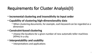
Requirements for Cluster Analysis(II)
• Incremental clustering and insensitivity to input order
• Capability of clustering high-dimensionality data
―When clustering documents, for example, each keyword can be regarded as a
dimension
• Constraint-based clustering
―choose the locations for a given number of new automatic teller machines
(ATMs) in a city.
• Interpretability and usability
―interpretations and applications

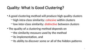
6. Quality: What Is Good Clustering?
• A good clustering method will produce high quality clusters
―high intra-class similarity: cohesive within clusters
―low inter-class similarity: distinctive between clusters
• The quality of a clustering method depends on
―the similarity measure used by the method
―its implementation, and
―Its ability to discover some or all of the hidden patterns
6

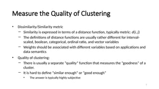
7. Measure the Quality of Clustering
• Dissimilarity/Similarity metric
― Similarity is expressed in terms of a distance function, typically metric: d(i, j)
― The definitions of distance functions are usually rather different for interval-
scaled, boolean, categorical, ordinal ratio, and vector variables
― Weights should be associated with different variables based on applications and
data semantics
• Quality of clustering:
― There is usually a separate “quality” function that measures the “goodness” of a
cluster.
― It is hard to define “similar enough” or “good enough”
• The answer is typically highly subjective
7

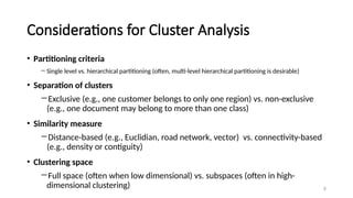
8. Considerations for Cluster Analysis
• Partitioning criteria
―Single level vs. hierarchical partitioning (often, multi-level hierarchical partitioning is desirable)
• Separation of clusters
―Exclusive (e.g., one customer belongs to only one region) vs. non-exclusive
(e.g., one document may belong to more than one class)
• Similarity measure
―Distance-based (e.g., Euclidian, road network, vector) vs. connectivity-based
(e.g., density or contiguity)
• Clustering space
―Full space (often when low dimensional) vs. subspaces (often in high-
dimensional clustering) 8

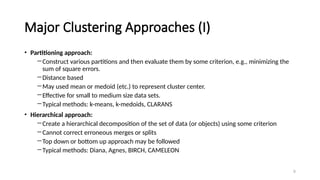
9. Major Clustering Approaches (I)
• Partitioning approach:
―Construct various partitions and then evaluate them by some criterion, e.g., minimizing the
sum of square errors.
―Distance based
―May used mean or medoid (etc.) to represent cluster center.
―Effective for small to medium size data sets.
―Typical methods: k-means, k-medoids, CLARANS
• Hierarchical approach:
―Create a hierarchical decomposition of the set of data (or objects) using some criterion
―Cannot correct erroneous merges or splits
―Top down or bottom up approach may be followed
―Typical methods: Diana, Agnes, BIRCH, CAMELEON
9

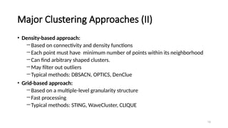
10. Major Clustering Approaches (II)
• Density-based approach:
―Based on connectivity and density functions
―Each point must have minimum number of points within its neighborhood
―Can find arbitrary shaped clusters.
―May filter out outliers
―Typical methods: DBSACN, OPTICS, DenClue
• Grid-based approach:
―Based on a multiple-level granularity structure
―Fast processing
―Typical methods: STING, WaveCluster, CLIQUE
10

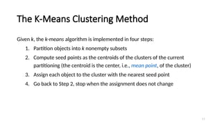
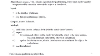
11. The K-Means Clustering Method
Given k, the k-means algorithm is implemented in four steps:
1. Partition objects into k nonempty subsets
2. Compute seed points as the centroids of the clusters of the current
partitioning (the centroid is the center, i.e., mean point, of the cluster)
3. Assign each object to the cluster with the nearest seed point
4. Go back to Step 2, stop when the assignment does not change
11

12. 12

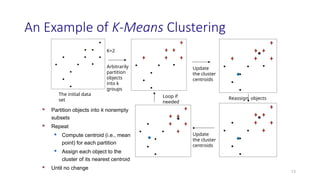
13. An Example of K-Means Clustering
13
K=2
Arbitrarily
partition
objects
into k
groups
Update
the cluster
centroids
Update
the cluster
centroids
Reassign objects
Loop if
needed
The initial data
set
 Partition objects into k nonempty
subsets
 Repeat
 Compute centroid (i.e., mean
point) for each partition
 Assign each object to the
cluster of its nearest centroid
 Until no change

14. 14
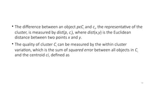
• The difference between an object pϵCi and ci, the representative of the
cluster, is measured by dist(p, ci), where dist(x,y) is the Euclidean
distance between two points x and y.
• The quality of cluster Ci can be measured by the within cluster
variation, which is the sum of squared error between all objects in Ci
and the centroid ci, defined as

15. 15
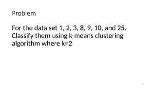
Problem
For the data set 1, 2, 3, 8, 9, 10, and 25.
Classify them using k-means clustering
algorithm where k=2

16. 16
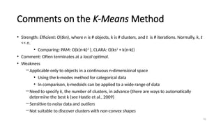
Comments on the K-Means Method
• Strength: Efficient: O(tkn), where n is # objects, k is # clusters, and t is # iterations. Normally, k, t
<< n.
• Comparing: PAM: O(k(n-k)2
), CLARA: O(ks2
+ k(n-k))
• Comment: Often terminates at a local optimal.
• Weakness
―Applicable only to objects in a continuous n-dimensional space
• Using the k-modes method for categorical data
• In comparison, k-medoids can be applied to a wide range of data
―Need to specify k, the number of clusters, in advance (there are ways to automatically
determine the best k (see Hastie et al., 2009)
―Sensitive to noisy data and outliers
―Not suitable to discover clusters with non-convex shapes

17. 17
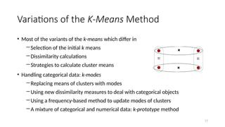
Variations of the K-Means Method
• Most of the variants of the k-means which differ in
―Selection of the initial k means
―Dissimilarity calculations
―Strategies to calculate cluster means
• Handling categorical data: k-modes
―Replacing means of clusters with modes
―Using new dissimilarity measures to deal with categorical objects
―Using a frequency-based method to update modes of clusters
―A mixture of categorical and numerical data: k-prototype method

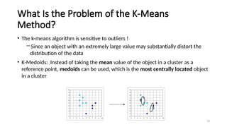
18. What Is the Problem of the K-Means
Method?
• The k-means algorithm is sensitive to outliers !
―Since an object with an extremely large value may substantially distort the
distribution of the data
• K-Medoids: Instead of taking the mean value of the object in a cluster as a
reference point, medoids can be used, which is the most centrally located object
in a cluster
18
0
1
2
3
4
5
6
7
8
9
10
0 1 2 3 4 5 6 7 8 9 10
0
1
2
3
4
5
6
7
8
9
10
0 1 2 3 4 5 6 7 8 9 10

19. 19

20. 20
Hierarchical Methods
20

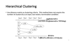
21. Hierarchical Clustering
• Use distance matrix as clustering criteria. This method does not require the
number of clusters k as an input, but needs a termination condition
21
Step 0 Step 1 Step 2 Step 3 Step 4
b
d
c
e
a a b
d e
c d e
a b c d e
Step 4 Step 3 Step 2 Step 1 Step 0
agglomerative
(AGNES-AGglomerative NESting)
divisive
(DIANA-DIvisive ANAlysis)

22. AGNES (Agglomerative Nesting)
• Introduced in Kaufmann and Rousseeuw (1990)
• Use the single-link method and the dissimilarity matrix
―Each cluster is represented by all the objects in the cluster, and the similarity between two
clusters is measured by the similarity of the closest pair of data points belonging to different
clusters.
• Merge nodes that have the least dissimilarity
• Go on in a non-descending fashion
• Eventually all nodes belong to the same cluster
22

23. DIANA (DIvisive ANAlysis)
• Introduced in Kaufmann and Rousseeuw (1990)
• Inverse order of AGNES
• Eventually each node forms a cluster on its own
• All the objects are used to form one initial cluster.
• The cluster is split according to some principle such as the maximum Euclidean
distance between the closest neighboring objects in the cluster.
• The cluster-splitting process repeats until, eventually, each new cluster contains
only a single object.
23

24. 24
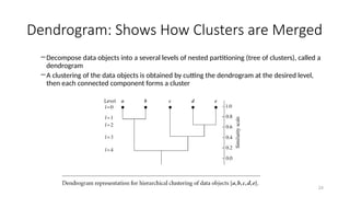
Dendrogram: Shows How Clusters are Merged
―Decompose data objects into a several levels of nested partitioning (tree of clusters), called a
dendrogram
―A clustering of the data objects is obtained by cutting the dendrogram at the desired level,
then each connected component forms a cluster

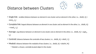
25. Distance between Clusters
• Single link: smallest distance between an element in one cluster and an element in the other, i.e., dist(Ki, Kj) =
min(tip, tjq)
• Complete link: largest distance between an element in one cluster and an element in the other, i.e., dist(Ki, Kj)
= max(tip, tjq)
• Average: avg distance between an element in one cluster and an element in the other, i.e., dist(Ki, Kj) = avg(tip,
tjq)
• Centroid: distance between the centroids of two clusters, i.e., dist(Ki, Kj) = dist(Ci, Cj)
• Medoid: distance between the medoids of two clusters, i.e., dist(Ki, Kj) = dist(Mi, Mj)
―Medoid: a chosen, centrally located object in the cluster
X X
25

26. 26
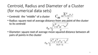
Centroid, Radius and Diameter of a Cluster
(for numerical data sets)
• Centroid: the “middle” of a cluster
• Radius: square root of average distance from any point of the cluster
to its centroid
• Diameter: square root of average mean squared distance between all
pairs of points in the cluster
N
t
N
i ip
m
C
)
(
1



)
1
(
2
)
(
1
1







N
N
iq
t
ip
t
N
i
N
i
m
D
N
m
c
ip
t
N
i
m
R
2
)
(
1





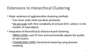
27. Extensions to Hierarchical Clustering
• Major weakness of agglomerative clustering methods
―Can never undo what was done previously
―Do not scale well: time complexity of at least O(n2
), where n is the
number of total objects
• Integration of hierarchical & distance-based clustering
―BIRCH (1996): uses CF-tree and incrementally adjusts the quality
of sub-clusters
―CHAMELEON (1999): hierarchical clustering using dynamic
modeling
27

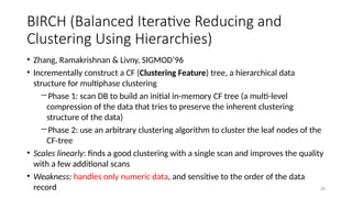
28. BIRCH (Balanced Iterative Reducing and
Clustering Using Hierarchies)
• Zhang, Ramakrishnan & Livny, SIGMOD’96
• Incrementally construct a CF (Clustering Feature) tree, a hierarchical data
structure for multiphase clustering
―Phase 1: scan DB to build an initial in-memory CF tree (a multi-level
compression of the data that tries to preserve the inherent clustering
structure of the data)
―Phase 2: use an arbitrary clustering algorithm to cluster the leaf nodes of the
CF-tree
• Scales linearly: finds a good clustering with a single scan and improves the quality
with a few additional scans
• Weakness: handles only numeric data, and sensitive to the order of the data
record 28

29. BIRCH (Balanced Iterative Reducing and
Clustering Using Hierarchies)
• BIRCH uses the notions of clustering feature to summarize a cluster,
and clustering feature tree (CF-tree) to represent a cluster hierarchy.
• These structures help the clustering method achieve good speed and
scalability in large or even streaming databases, and also make it
effective for incremental and dynamic clustering of incoming objects.
29

30. 30
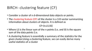
BIRCH- clustering feature (CF)
• Consider a cluster of n d-dimensional data objects or points.
• The clustering feature (CF) of the cluster is a 3-D vector summarizing
information about clusters of objects. It is defined as
CF={n,LS,SS}
• Where LS is the linear sum of the n points (i.e, and SS is the square
sum of the data points (i.e.
• A clustering feature is essentially a summary of the statistics for the
given cluster.Using a clustering feature, we can easily derive many
useful statistics of a cluster

31. 31
BIRCH
• the cluster’s centroid, x0, radius, R, and diameter, D, are

32. 32
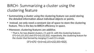
BIRCH- Summarizing a cluster using the
clustering feature
• Summarizing a cluster using the clustering feature can avoid storing
the detailed information about individual objects or points.
• Instead, we only need a constant size of space to store the clustering
feature. This is the key to BIRCH efficiency in space.
• Moreover, clustering features are additive.
―That is, for two disjoint clusters, C1 and C2, with the clustering features
CF1={n1,LS1,SS1} and CF2={n2,LS2,SS2}, respectively, the clustering feature for
the cluster that formed by merging C1 and C2 is simply
CF1+CF2 ={n1+n2,LS1+LS2,SS1+SS2}.

33. 33
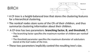
BIRCH
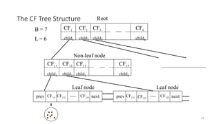
• A CF-tree is a height-balanced tree that stores the clustering features
for a hierarchical clustering.
• The nonleaf nodes store sums of the CFs of their children, and thus
summarize clustering information about their children.
• A CF-tree has two parameters: branching factor, B, and threshold, T.
―The branching factor specifies the maximum number of children per nonleaf
node.
―The threshold parameter specifies the maximum diameter of subclusters
stored at the leaf nodes of the tree.
• These two parameters implicitly control the resulting tree’s size.

34. The CF Tree Structure
34
CF1
child1
CF3
child3
CF2
child2
CF6
child6
CF11
child1
CF13
child3
CF12
child2
CF15
child5
CF111 CF112 CF116
prev next CF121 CF122
CF124
prev next
B = 7
L = 6
Root
Non-leaf node
Leaf node Leaf node

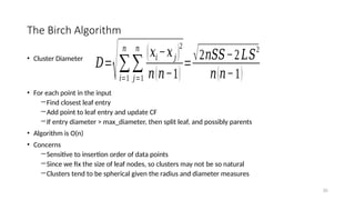
35. The Birch Algorithm
• Cluster Diameter
• For each point in the input
―Find closest leaf entry
―Add point to leaf entry and update CF
―If entry diameter > max_diameter, then split leaf, and possibly parents
• Algorithm is O(n)
• Concerns
―Sensitive to insertion order of data points
―Since we fix the size of leaf nodes, so clusters may not be so natural
―Clusters tend to be spherical given the radius and diameter measures
35
𝐷=
√∑
𝑖=1
𝑛
∑
𝑗=1
𝑛
(𝑥𝑖−𝑥𝑗 )
2
𝑛(𝑛−1)
=√2𝑛𝑆𝑆−2𝐿𝑆
2
𝑛(𝑛−1)

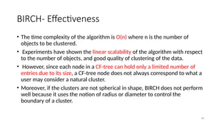
36. 36
BIRCH- Effectiveness
• The time complexity of the algorithm is O(n) where n is the number of
objects to be clustered.
• Experiments have shown the linear scalability of the algorithm with respect
to the number of objects, and good quality of clustering of the data.
• However, since each node in a CF-tree can hold only a limited number of
entries due to its size, a CF-tree node does not always correspond to what a
user may consider a natural cluster.
• Moreover, if the clusters are not spherical in shape, BIRCH does not perform
well because it uses the notion of radius or diameter to control the
boundary of a cluster.

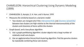
37. CHAMELEON: Hierarchical Clustering Using Dynamic Modeling
(1999)
• CHAMELEON: G. Karypis, E. H. Han, and V. Kumar, 1999
• Measures the similarity based on a dynamic model
― Two clusters are merged only if the interconnectivity and closeness (proximity)
between two clusters are high relative to the internal interconnectivity of the
clusters and closeness of items within the clusters
• Graph-based, and a two-phase algorithm
1. Use a graph-partitioning algorithm: cluster objects into a large number of
relatively small sub-clusters
2. Use an agglomerative hierarchical clustering algorithm: find the genuine clusters
by repeatedly combining these sub-clusters
37

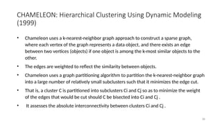
38. CHAMELEON: Hierarchical Clustering Using Dynamic Modeling
(1999)
• Chameleon uses a k-nearest-neighbor graph approach to construct a sparse graph,
where each vertex of the graph represents a data object, and there exists an edge
between two vertices (objects) if one object is among the k-most similar objects to the
other.
• The edges are weighted to reflect the similarity between objects.
• Chameleon uses a graph partitioning algorithm to partition the k-nearest-neighbor graph
into a large number of relatively small subclusters such that it minimizes the edge cut.
• That is, a cluster C is partitioned into subclusters Ci and Cj so as to minimize the weight
of the edges that would be cut should C be bisected into Ci and Cj .
• It assesses the absolute interconnectivity between clusters Ci and Cj .
38

39. CHAMELEON
• Chameleon then uses an agglomerative hierarchical clustering algorithm that
iteratively merges subclusters based on their similarity.
• To determine the pairs of most similar subclusters, it takes into account both
the interconnectivity and the closeness of the clusters.
• Specifically, Chameleon determines the similarity between each pair of clusters
Ci and Cj according to their relative interconnectivity, RI(Ci ,Cj), and their
relative closeness,RC(Ci ,Cj).
39

40. 40
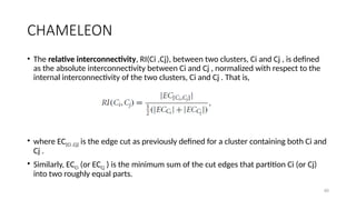
CHAMELEON
• The relative interconnectivity, RI(Ci ,Cj), between two clusters, Ci and Cj , is defined
as the absolute interconnectivity between Ci and Cj , normalized with respect to the
internal interconnectivity of the two clusters, Ci and Cj . That is,
• where EC{Ci ,Cj} is the edge cut as previously defined for a cluster containing both Ci and
Cj .
• Similarly, ECCi (or ECCj ) is the minimum sum of the cut edges that partition Ci (or Cj)
into two roughly equal parts.

41. 41
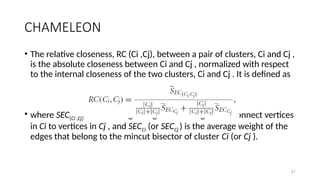
CHAMELEON
• The relative closeness, RC (Ci ,Cj), between a pair of clusters, Ci and Cj ,
is the absolute closeness between Ci and Cj , normalized with respect
to the internal closeness of the two clusters, Ci and Cj . It is defined as
• where SEC{Ci ,Cj} is the average weight of the edges that connect vertices
in Ci to vertices in Cj , and SECCi (or SECCj ) is the average weight of the
edges that belong to the mincut bisector of cluster Ci (or Cj ).

42. 42
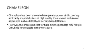
CHAMELEON
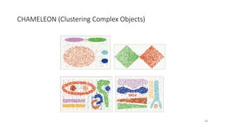
• Chameleon has been shown to have greater power at discovering
arbitrarily shaped clusters of high quality than several well-known
algorithms such as BIRCH and density based DBSCAN.
• However, the processing cost for high-dimensional data may require
O(n2
)time for n objects in the worst case.

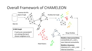
43. Overall Framework of CHAMELEON
43
Construct (K-NN)
Sparse Graph Partition the Graph
Merge Partition
Final Clusters
Data Set
K-NN Graph
P and q are connected if
q is among the top k
closest neighbors of p
Relative interconnectivity:
connectivity of c1 and c2
over internal connectivity
Relative closeness:
closeness of c1 and c2 over
internal closeness

44. CHAMELEON (Clustering Complex Objects)
44