The document discusses the importance of systematic data collection and classification for effective statistical analysis, outlining methods for organizing data into homogenous groups based on various criteria. It emphasizes the need for clarity and usefulness in data classification and tabulation, detailing different types of classifications such as geographical, chronological, qualitative, and quantitative. Additionally, the document covers the preparation of frequency distribution and cumulative frequency distribution tables to facilitate data interpretation.

2. The raw data collected through surveys or experiments
will be of no use if it is haphazard and unsystematic.
Because that data is not appropriate to draw conclusions
and make interpretations.
Hence it becomes important to arrange data into a
systematic form so as to identify the number of units
belonging to a particular classified group.
This enables the comparison and further statististical
treatment or analysis of data etc.

3. • The placement of data in different homogenous groups
formed on the basis of some characteristics or criteria is
called classification.
According to L. R. Connor
Classification is the process of arranging things (actually or
notionally) in groups or classes according to their resemblance
and affinities, and give expression to the unity of attributes that
may subsist amongst the diversity of individuals.

4. First of all every researcher or statistician should reduce and simplify the
details into forms so that the salient features may be brought out, while still
facilitating the interpretation of the assembled data.
 So table is a systematic arrangement of data in rows and/or column.
 Classification or tabulation mostly depend on type of information
required for study and type of further statistical treatment to be
undertaken.
1. The classes should be complete and non-overlapping. It means that each
observation or unit must belong to an unique class.
2. Clarity of classes is another important property. i.e. there should be no
confusion in placing a unit in a class.
3. One should use standardised class so that the comparison of unit become
possible.
Norms for ideal classification are:

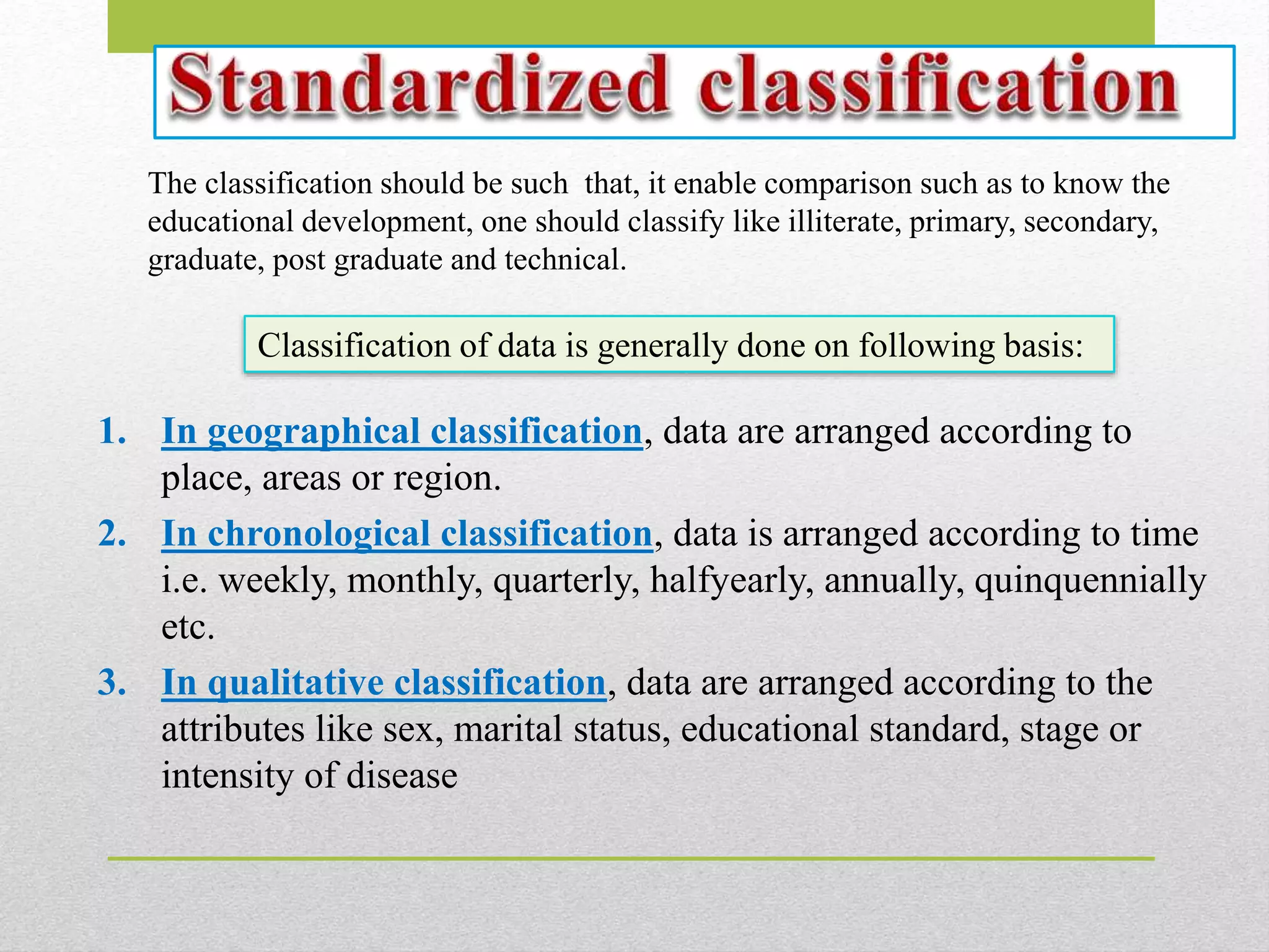
5. 1. In geographical classification, data are arranged according to
place, areas or region.
2. In chronological classification, data is arranged according to time
i.e. weekly, monthly, quarterly, halfyearly, annually, quinquennially
etc.
3. In qualitative classification, data are arranged according to the
attributes like sex, marital status, educational standard, stage or
intensity of disease
The classification should be such that, it enable comparison such as to know the
educational development, one should classify like illiterate, primary, secondary,
graduate, post graduate and technical.
Classification of data is generally done on following basis:

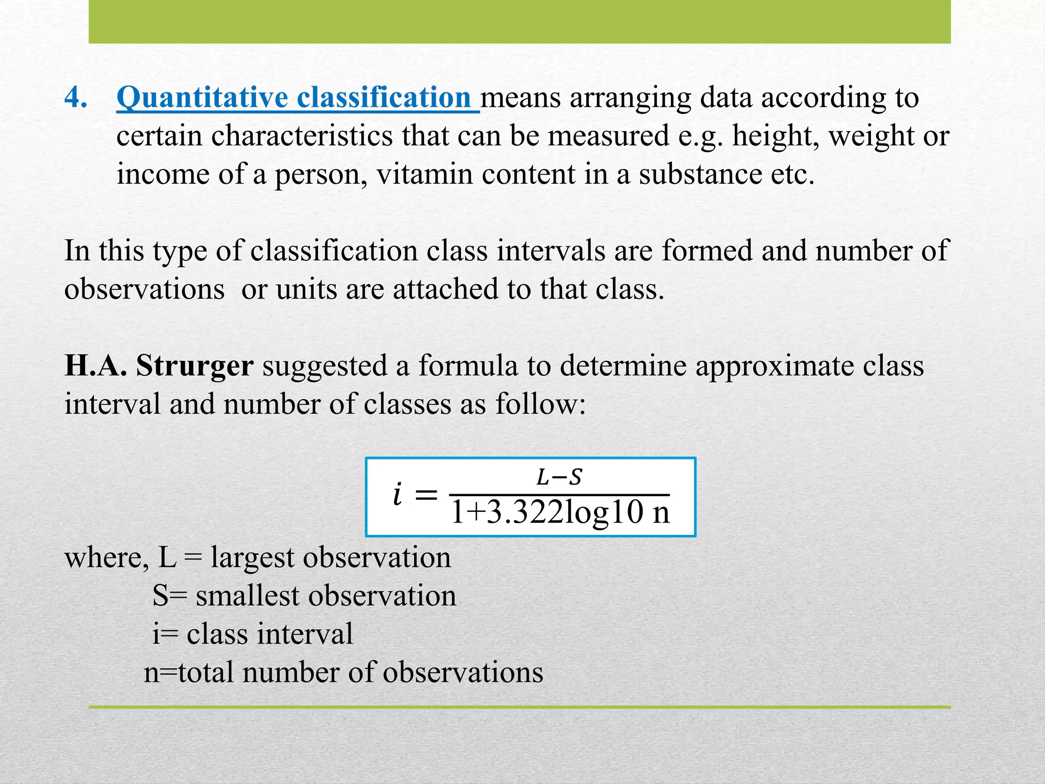
6. 4. Quantitative classification means arranging data according to
certain characteristics that can be measured e.g. height, weight or
income of a person, vitamin content in a substance etc.
In this type of classification class intervals are formed and number of
observations or units are attached to that class.
H.A. Strurger suggested a formula to determine approximate class
interval and number of classes as follow:
where, L = largest observation
S= smallest observation
i= class interval
n=total number of observations
𝑖 =
𝐿−𝑆
1+3.322log10 n

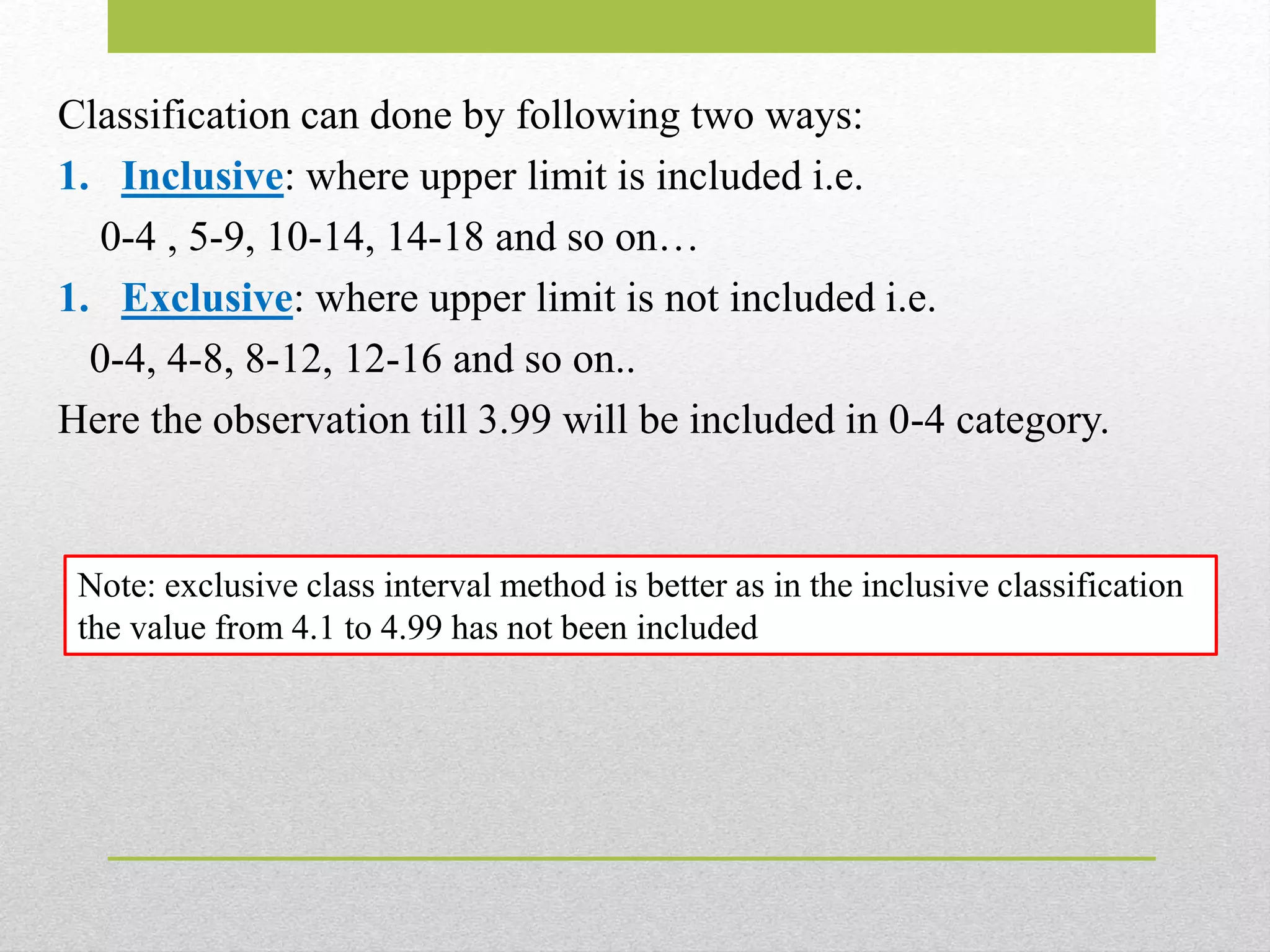
7. Classification can done by following two ways:
1. Inclusive: where upper limit is included i.e.
0-4 , 5-9, 10-14, 14-18 and so on…
1. Exclusive: where upper limit is not included i.e.
0-4, 4-8, 8-12, 12-16 and so on..
Here the observation till 3.99 will be included in 0-4 category.
Note: exclusive class interval method is better as in the inclusive classification
the value from 4.1 to 4.99 has not been included

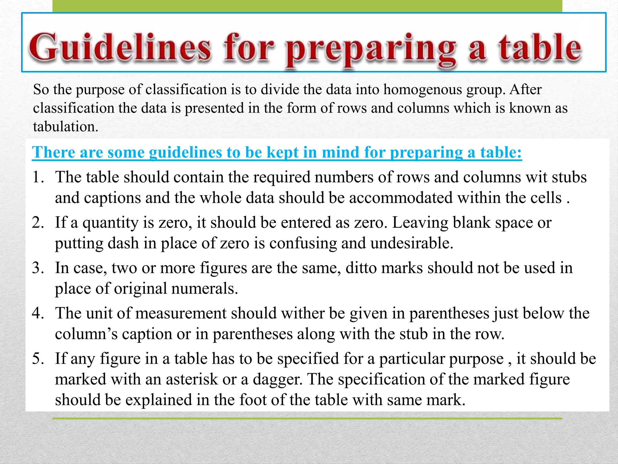
8. There are some guidelines to be kept in mind for preparing a table:
1. The table should contain the required numbers of rows and columns wit stubs
and captions and the whole data should be accommodated within the cells .
2. If a quantity is zero, it should be entered as zero. Leaving blank space or
putting dash in place of zero is confusing and undesirable.
3. In case, two or more figures are the same, ditto marks should not be used in
place of original numerals.
4. The unit of measurement should wither be given in parentheses just below the
column’s caption or in parentheses along with the stub in the row.
5. If any figure in a table has to be specified for a particular purpose , it should be
marked with an asterisk or a dagger. The specification of the marked figure
should be explained in the foot of the table with same mark.
So the purpose of classification is to divide the data into homogenous group. After
classification the data is presented in the form of rows and columns which is known as
tabulation.

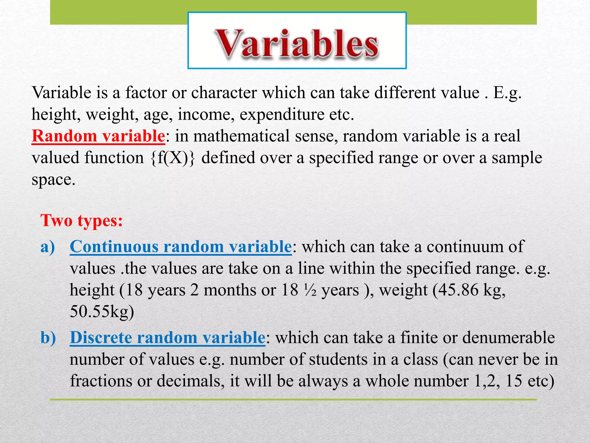
9. Two types:
a) Continuous random variable: which can take a continuum of
values .the values are take on a line within the specified range. e.g.
height (18 years 2 months or 18 ½ years ), weight (45.86 kg,
50.55kg)
b) Discrete random variable: which can take a finite or denumerable
number of values e.g. number of students in a class (can never be in
fractions or decimals, it will be always a whole number 1,2, 15 etc)
Variable is a factor or character which can take different value . E.g.
height, weight, age, income, expenditure etc.
Random variable: in mathematical sense, random variable is a real
valued function {f(X)} defined over a specified range or over a sample
space.

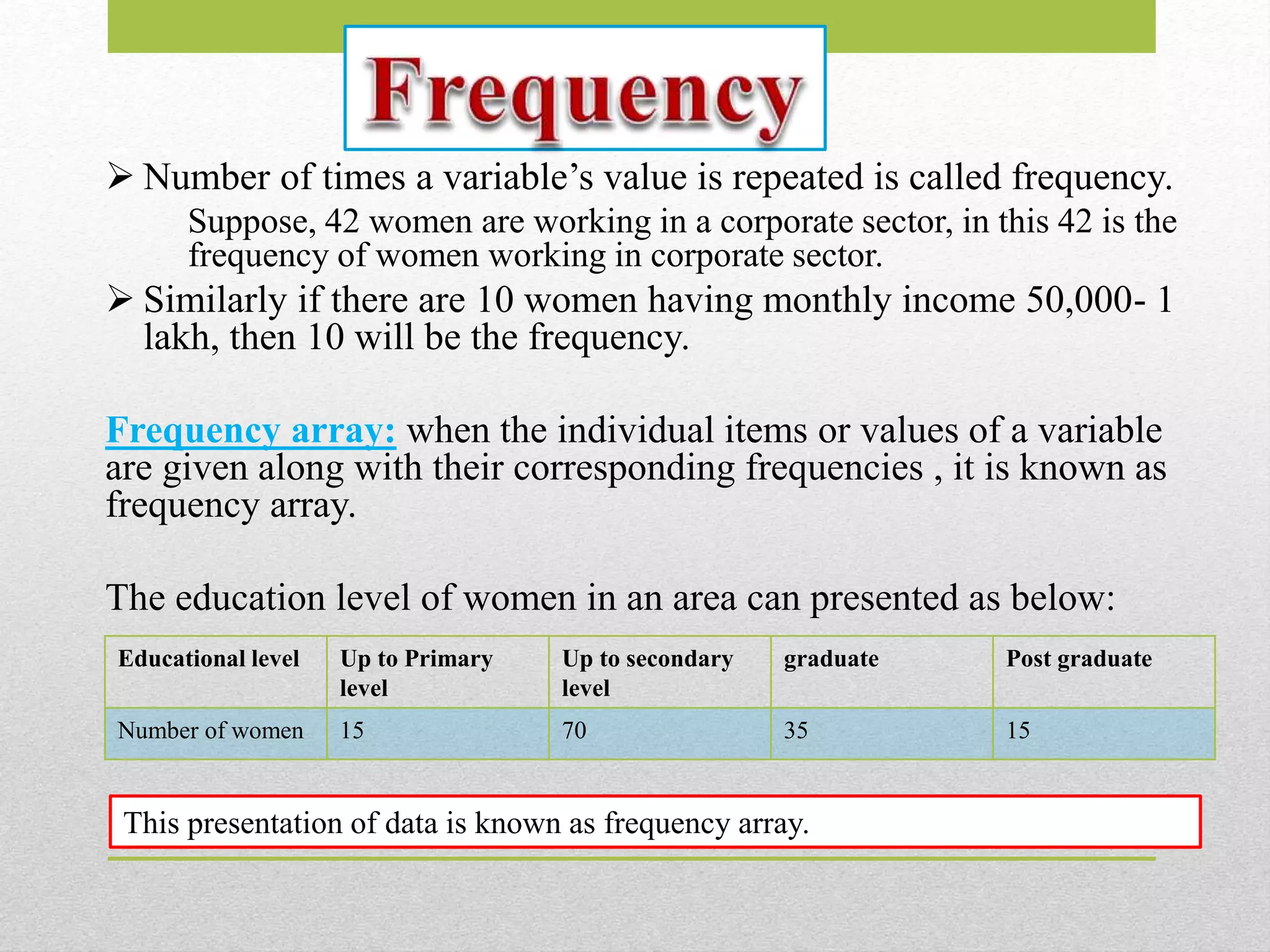
10.  Number of times a variable’s value is repeated is called frequency.
Suppose, 42 women are working in a corporate sector, in this 42 is the
frequency of women working in corporate sector.
 Similarly if there are 10 women having monthly income 50,000- 1
lakh, then 10 will be the frequency.
Frequency array: when the individual items or values of a variable
are given along with their corresponding frequencies , it is known as
frequency array.
The education level of women in an area can presented as below:
Educational level Up to Primary
level
Up to secondary
level
graduate Post graduate
Number of women 15 70 35 15
This presentation of data is known as frequency array.

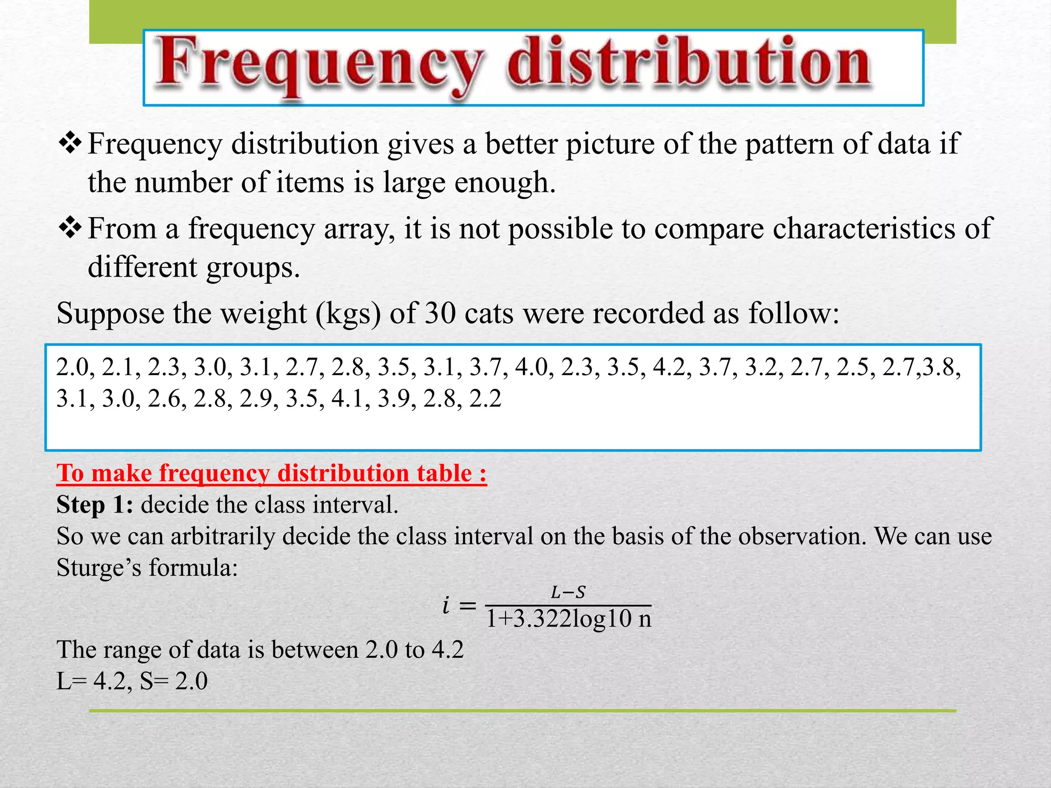
11. Frequency distribution gives a better picture of the pattern of data if
the number of items is large enough.
From a frequency array, it is not possible to compare characteristics of
different groups.
Suppose the weight (kgs) of 30 cats were recorded as follow:
2.0, 2.1, 2.3, 3.0, 3.1, 2.7, 2.8, 3.5, 3.1, 3.7, 4.0, 2.3, 3.5, 4.2, 3.7, 3.2, 2.7, 2.5, 2.7,3.8,
3.1, 3.0, 2.6, 2.8, 2.9, 3.5, 4.1, 3.9, 2.8, 2.2
To make frequency distribution table :
Step 1: decide the class interval.
So we can arbitrarily decide the class interval on the basis of the observation. We can use
Sturge’s formula:
𝑖 =
𝐿−𝑆
1+3.322log10 n
The range of data is between 2.0 to 4.2
L= 4.2, S= 2.0

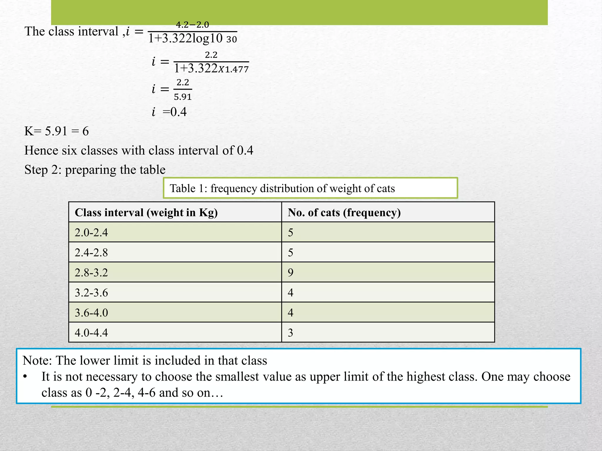
12. The class interval ,𝑖 =
4.2−2.0
1+3.322log10 30
𝑖 =
2.2
1+3.322 𝑋1.477
𝑖 =
2.2
5.91
𝑖 =0.4
K= 5.91 = 6
Hence six classes with class interval of 0.4
Step 2: preparing the table
Class interval (weight in Kg) No. of cats (frequency)
2.0-2.4 5
2.4-2.8 5
2.8-3.2 9
3.2-3.6 4
3.6-4.0 4
4.0-4.4 3
Table 1: frequency distribution of weight of cats
Note: The lower limit is included in that class
• It is not necessary to choose the smallest value as upper limit of the highest class. One may choose
class as 0 -2, 2-4, 4-6 and so on…

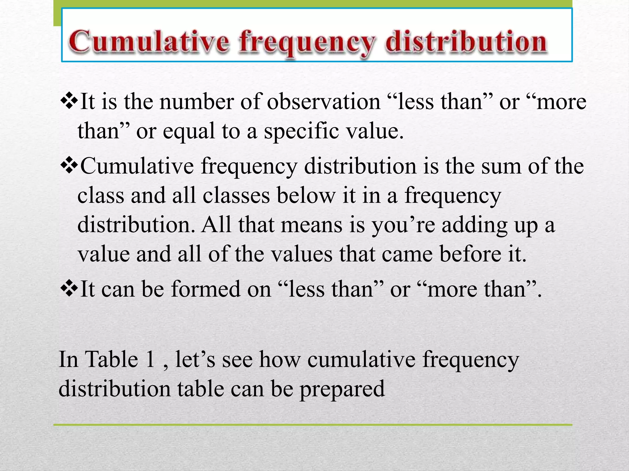
13. It is the number of observation “less than” or “more
than” or equal to a specific value.
Cumulative frequency distribution is the sum of the
class and all classes below it in a frequency
distribution. All that means is you’re adding up a
value and all of the values that came before it.
It can be formed on “less than” or “more than”.
In Table 1 , let’s see how cumulative frequency
distribution table can be prepared

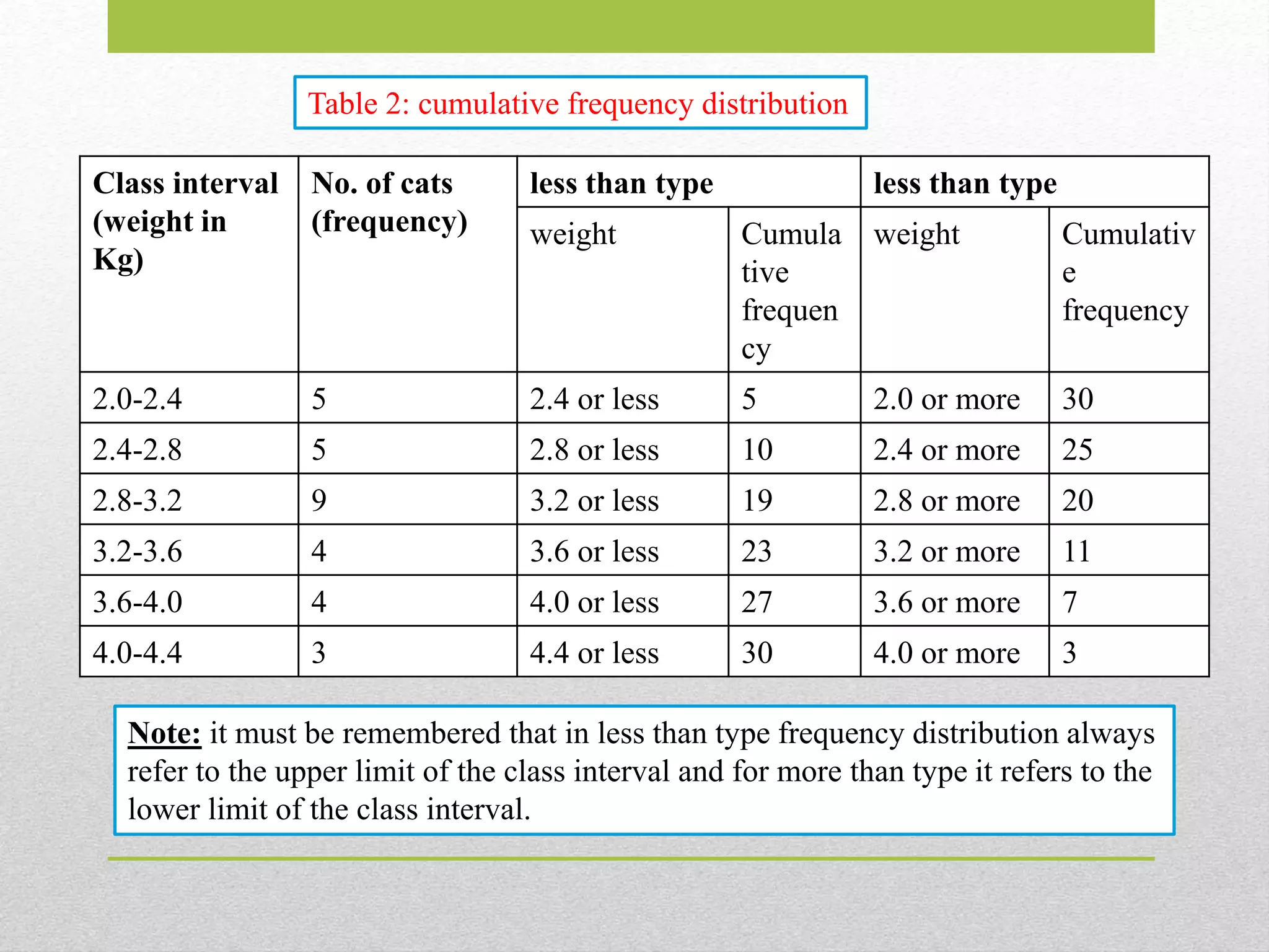
14. Class interval
(weight in
Kg)
No. of cats
(frequency)
less than type less than type
weight Cumula
tive
frequen
cy
weight Cumulativ
e
frequency
2.0-2.4 5 2.4 or less 5 2.0 or more 30
2.4-2.8 5 2.8 or less 10 2.4 or more 25
2.8-3.2 9 3.2 or less 19 2.8 or more 20
3.2-3.6 4 3.6 or less 23 3.2 or more 11
3.6-4.0 4 4.0 or less 27 3.6 or more 7
4.0-4.4 3 4.4 or less 30 4.0 or more 3
Note: it must be remembered that in less than type frequency distribution always
refer to the upper limit of the class interval and for more than type it refers to the
lower limit of the class interval.
Table 2: cumulative frequency distribution