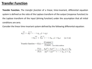
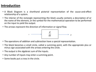
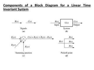
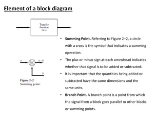
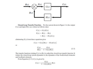
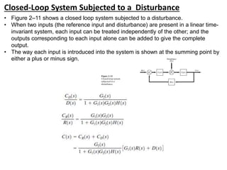
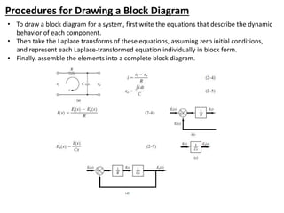
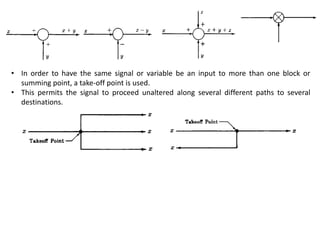
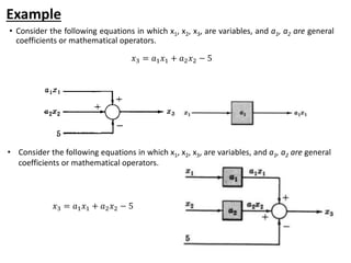
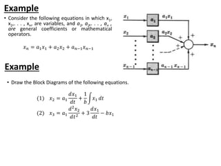
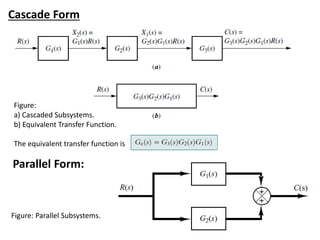
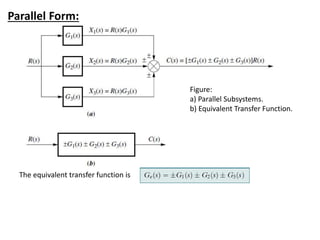
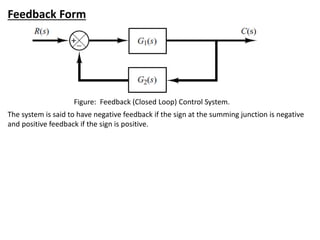
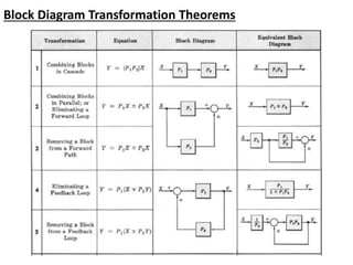
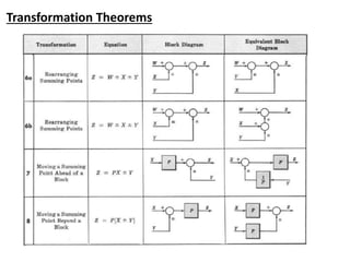
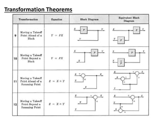
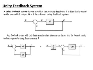
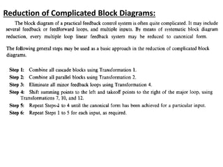
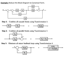
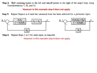
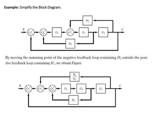
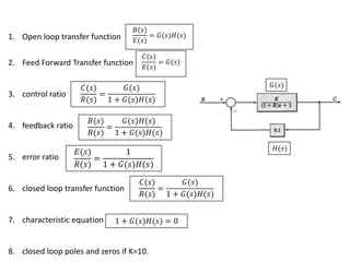
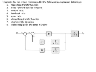
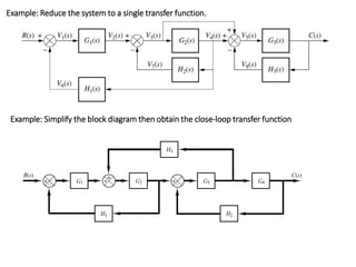
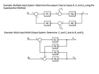
The document outlines the principles of biomedical control systems, focusing on block diagrams and their role in analyzing linear time-invariant systems. It describes key components such as transfer functions, summing points, branch points, and the significance of feedback in closed-loop systems. Additionally, it provides procedures for constructing block diagrams and examples to illustrate different configurations and transfer functions.
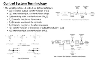


![Reduction of multiple subsystem [compatibility mode]](https://cdn.slidesharecdn.com/ss_thumbnails/reductionofmultiplesubsystemcompatibilitymode-110418075355-phpapp01-thumbnail.jpg?width=640&height=640&fit=bounds)