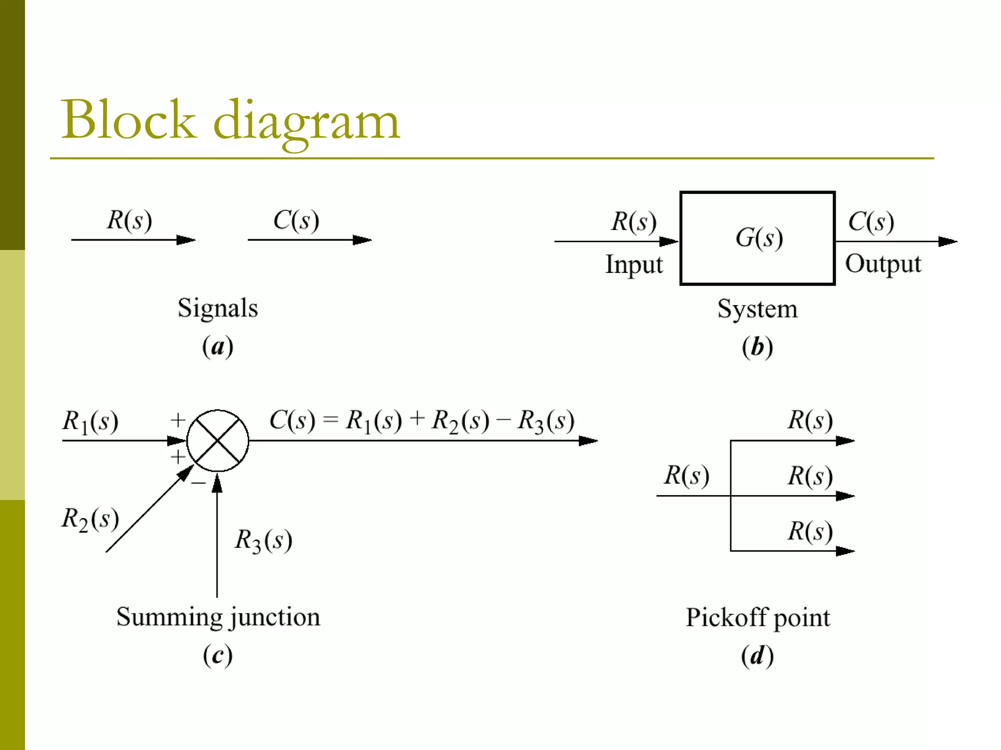
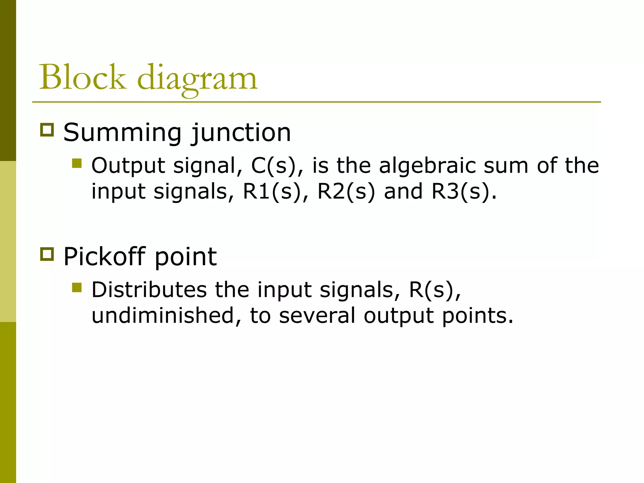
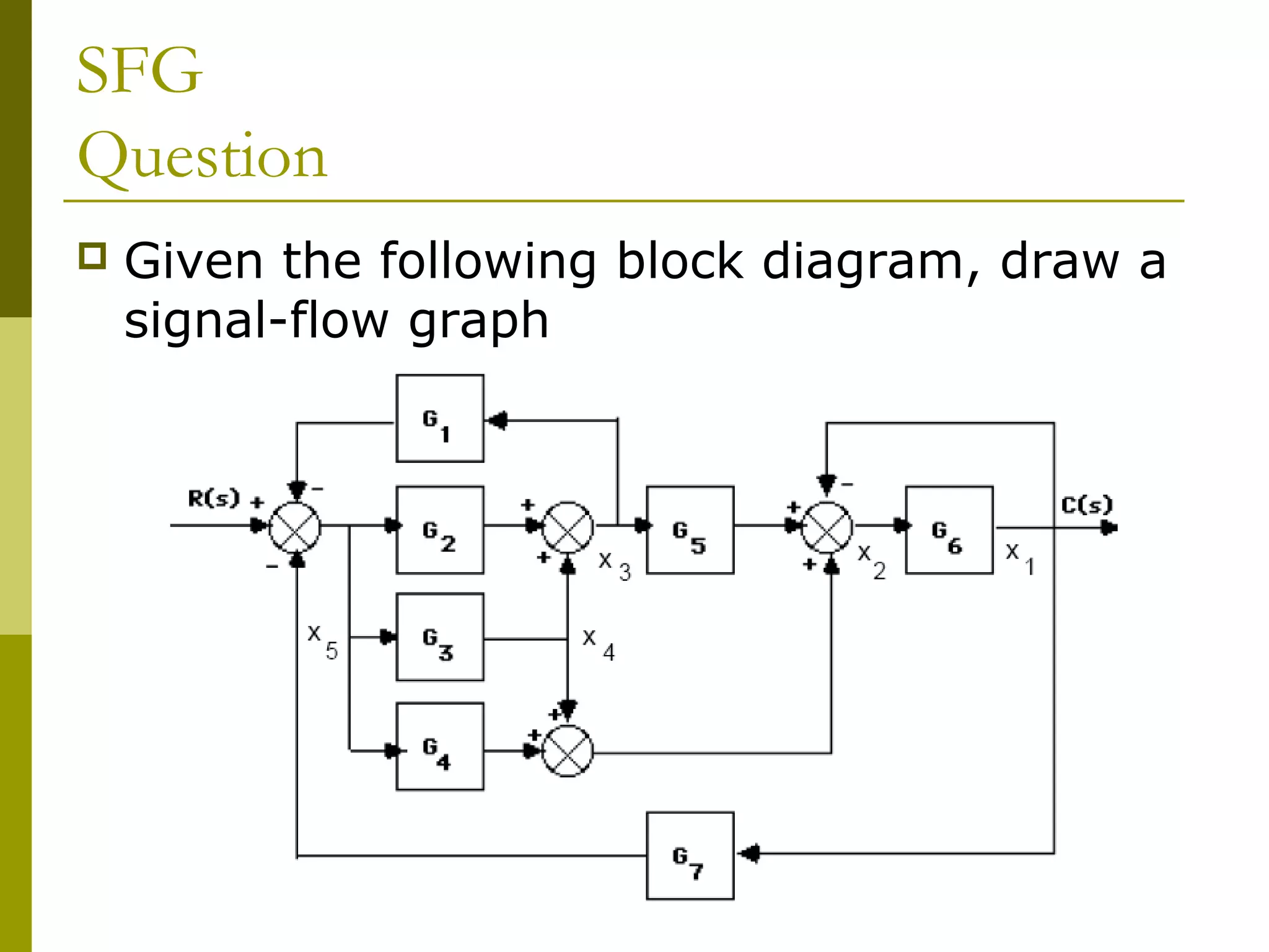
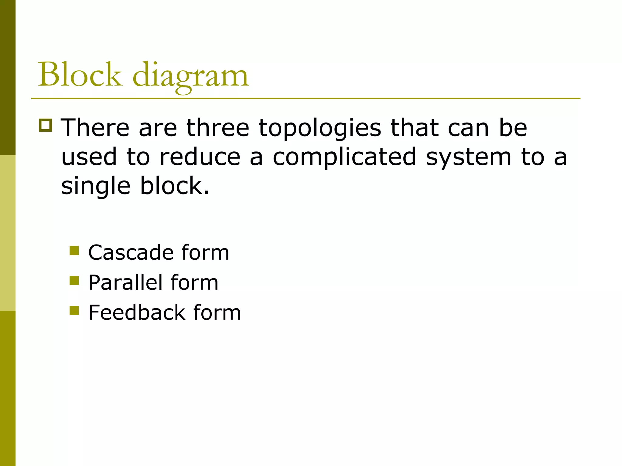
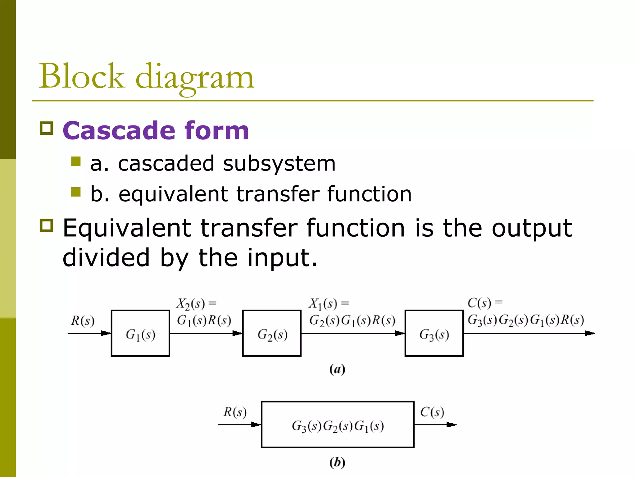
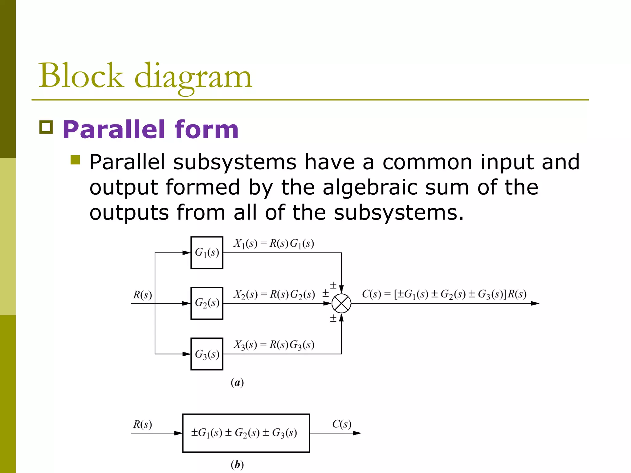
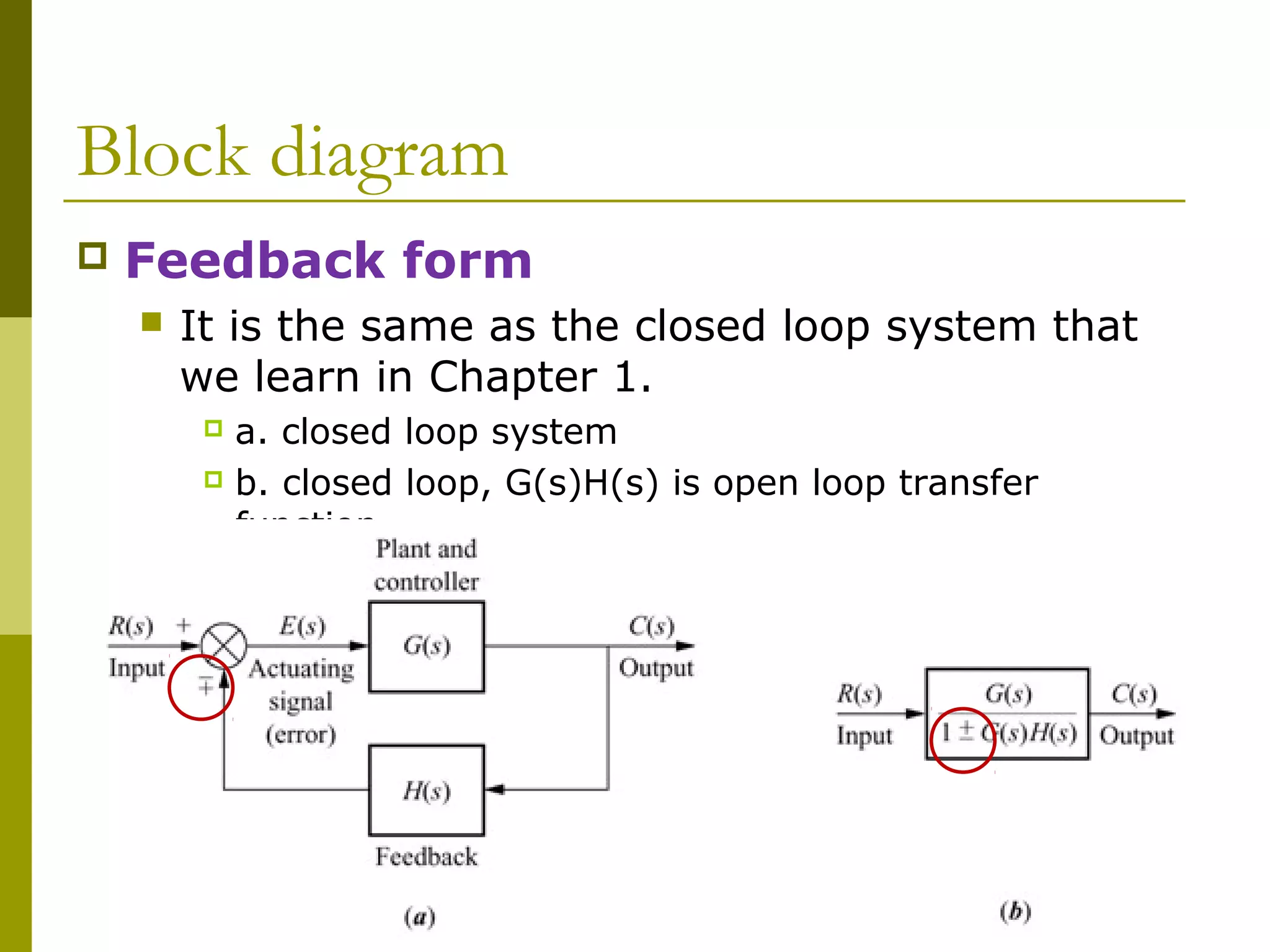
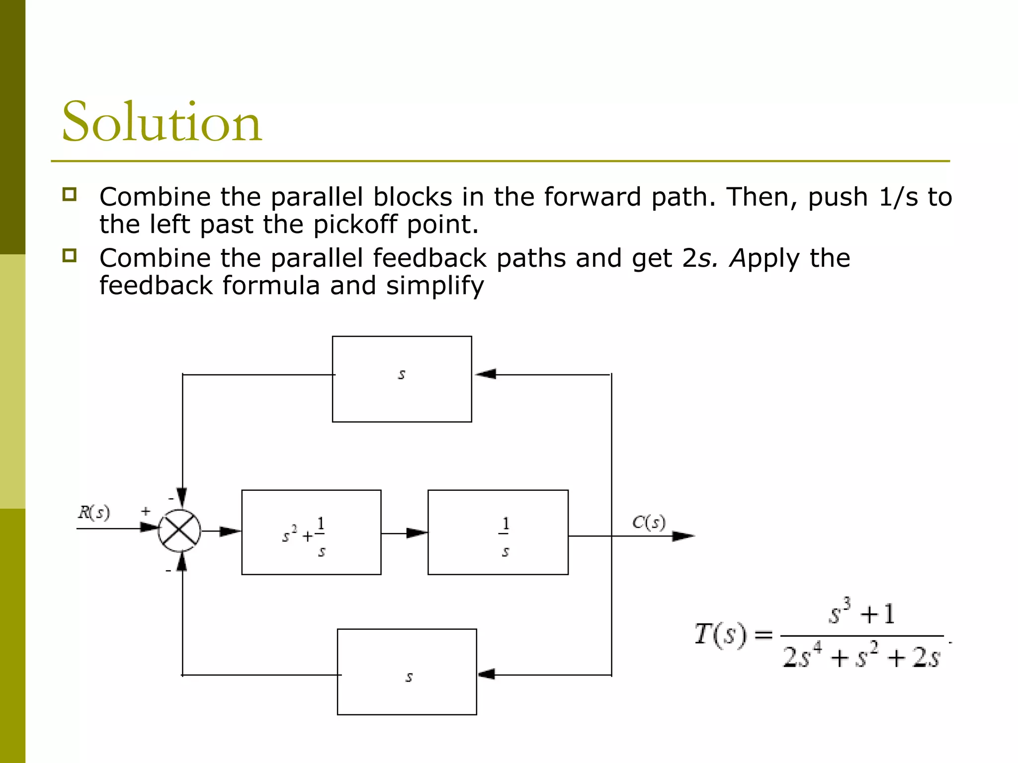
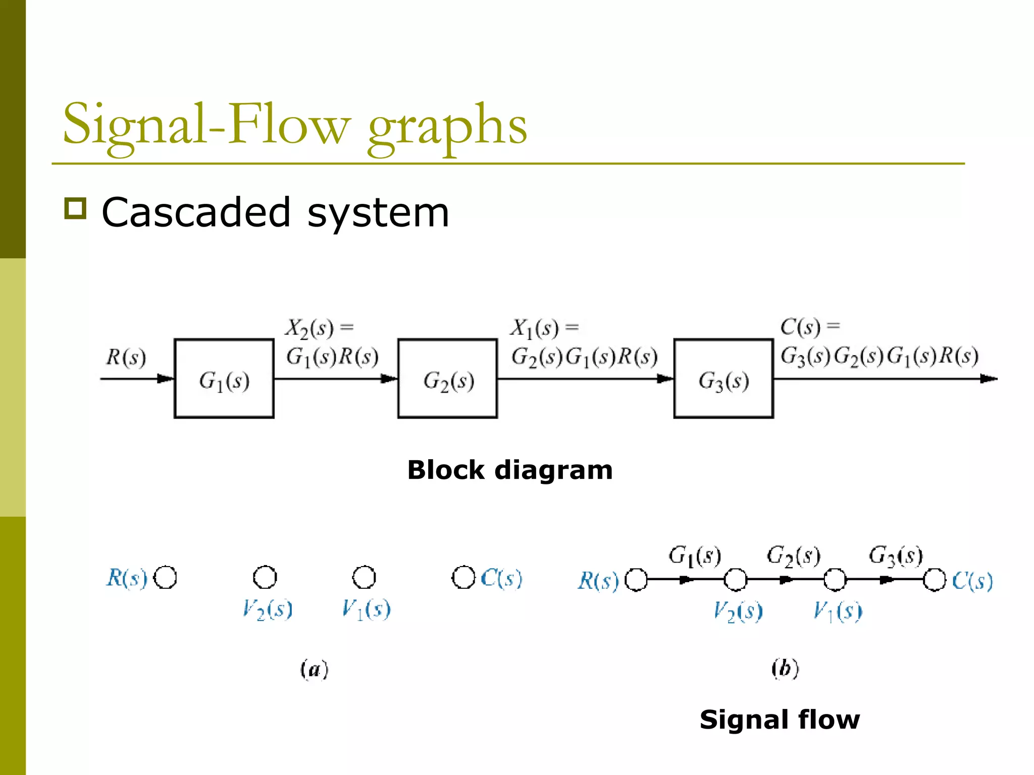
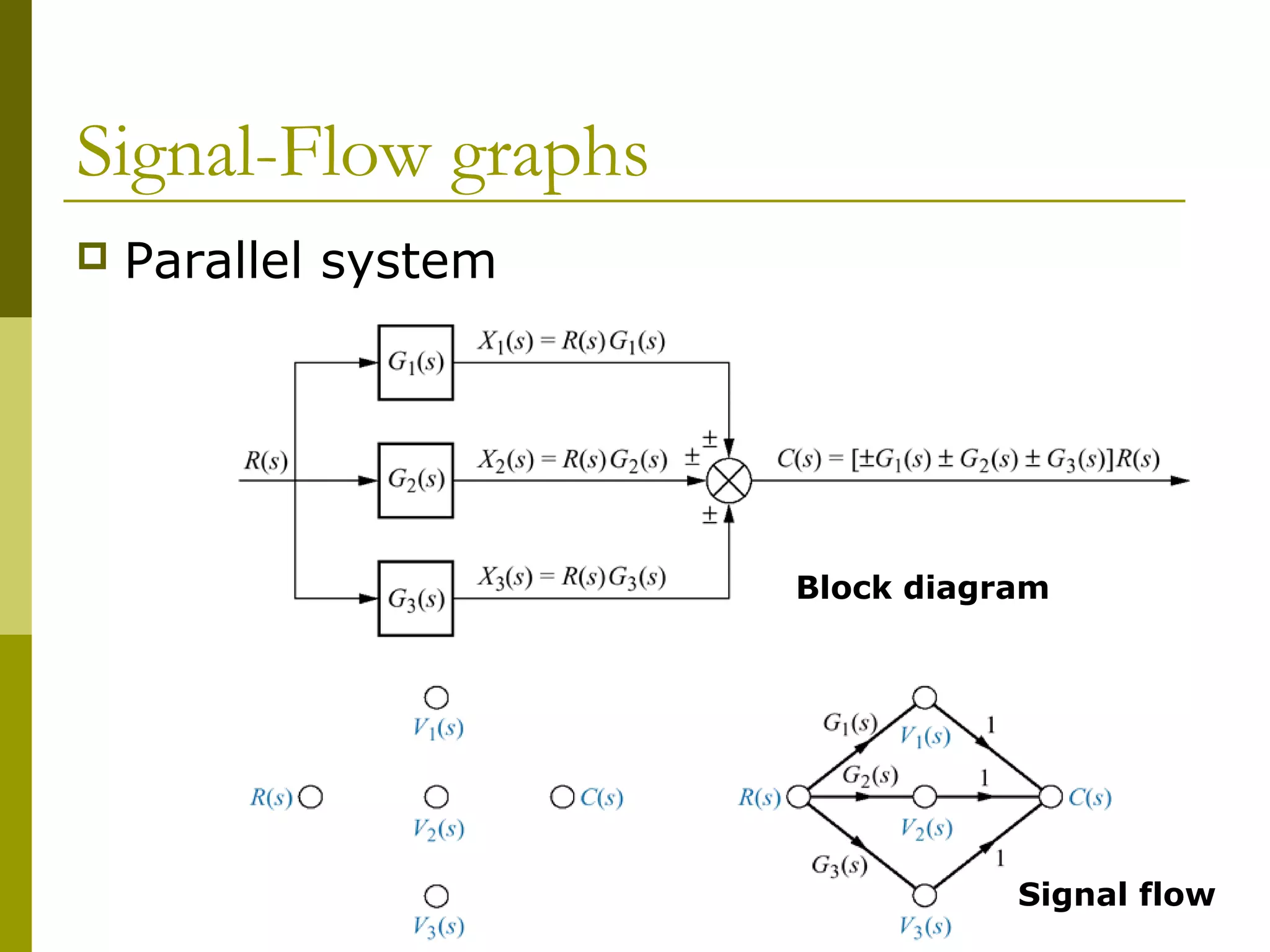
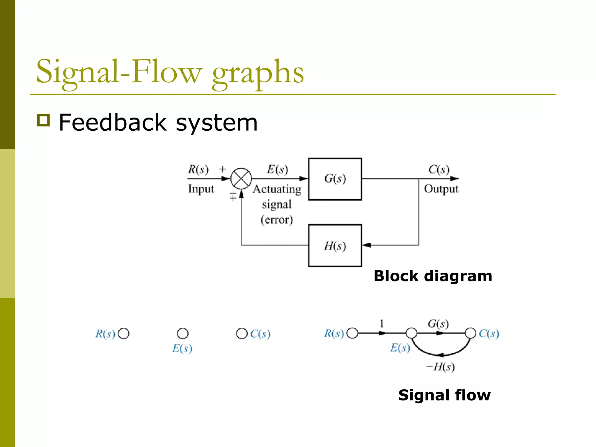
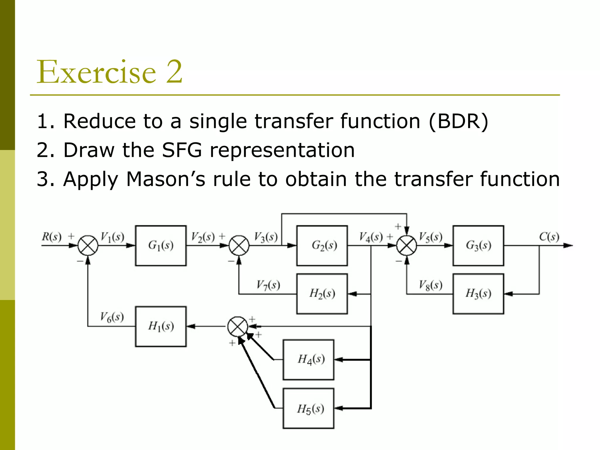
This document provides an overview of techniques for reducing block diagrams and signal flow graphs of multiple interconnected subsystems down to a single transfer function. It introduces common block diagram elements like summing junctions and pickoff points used to represent interconnections. 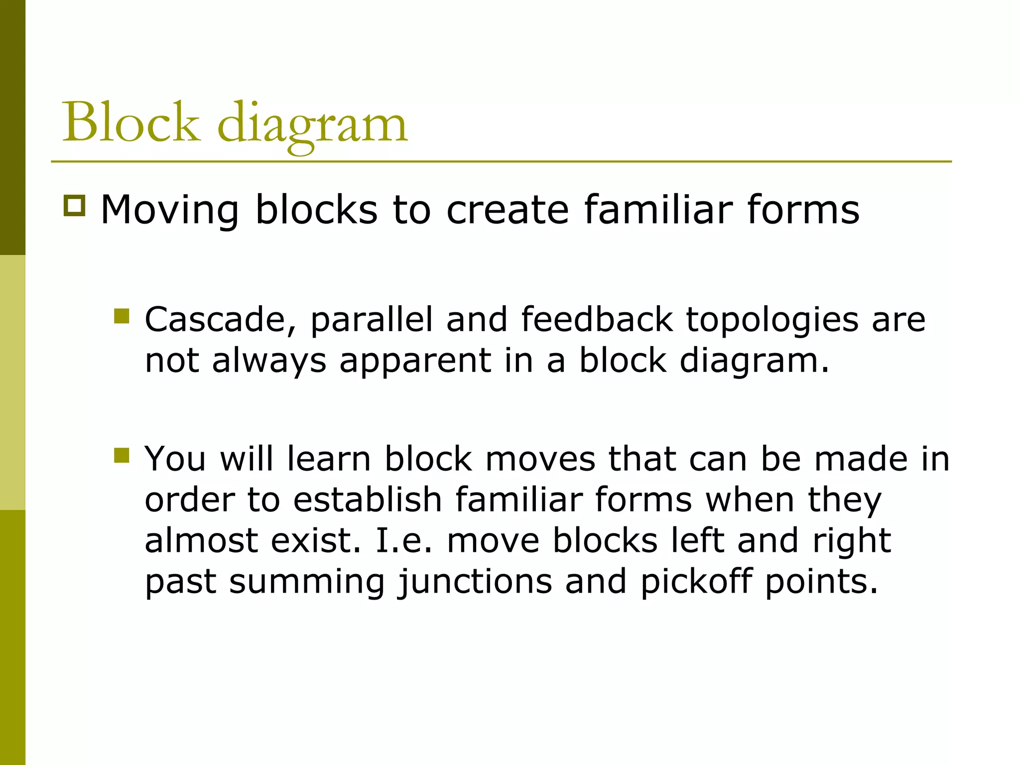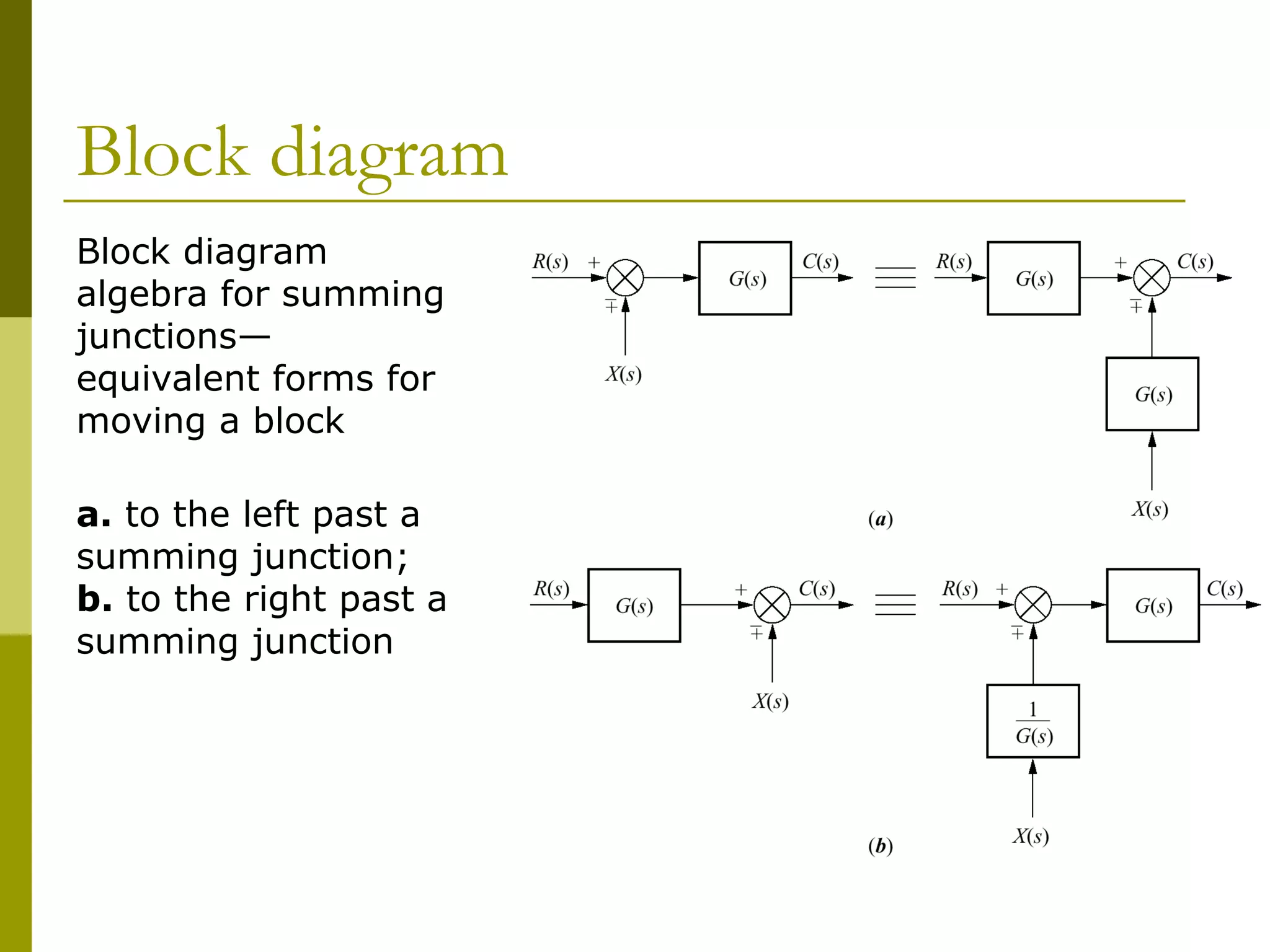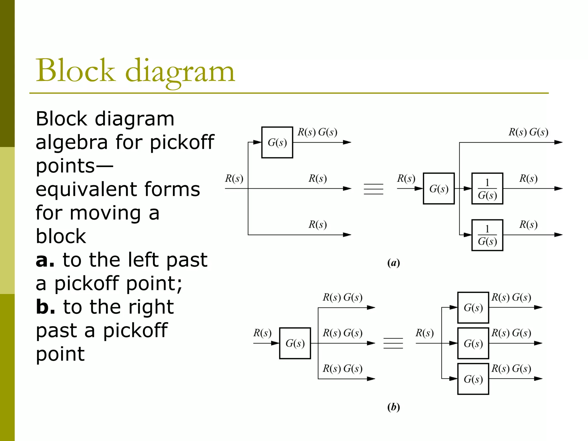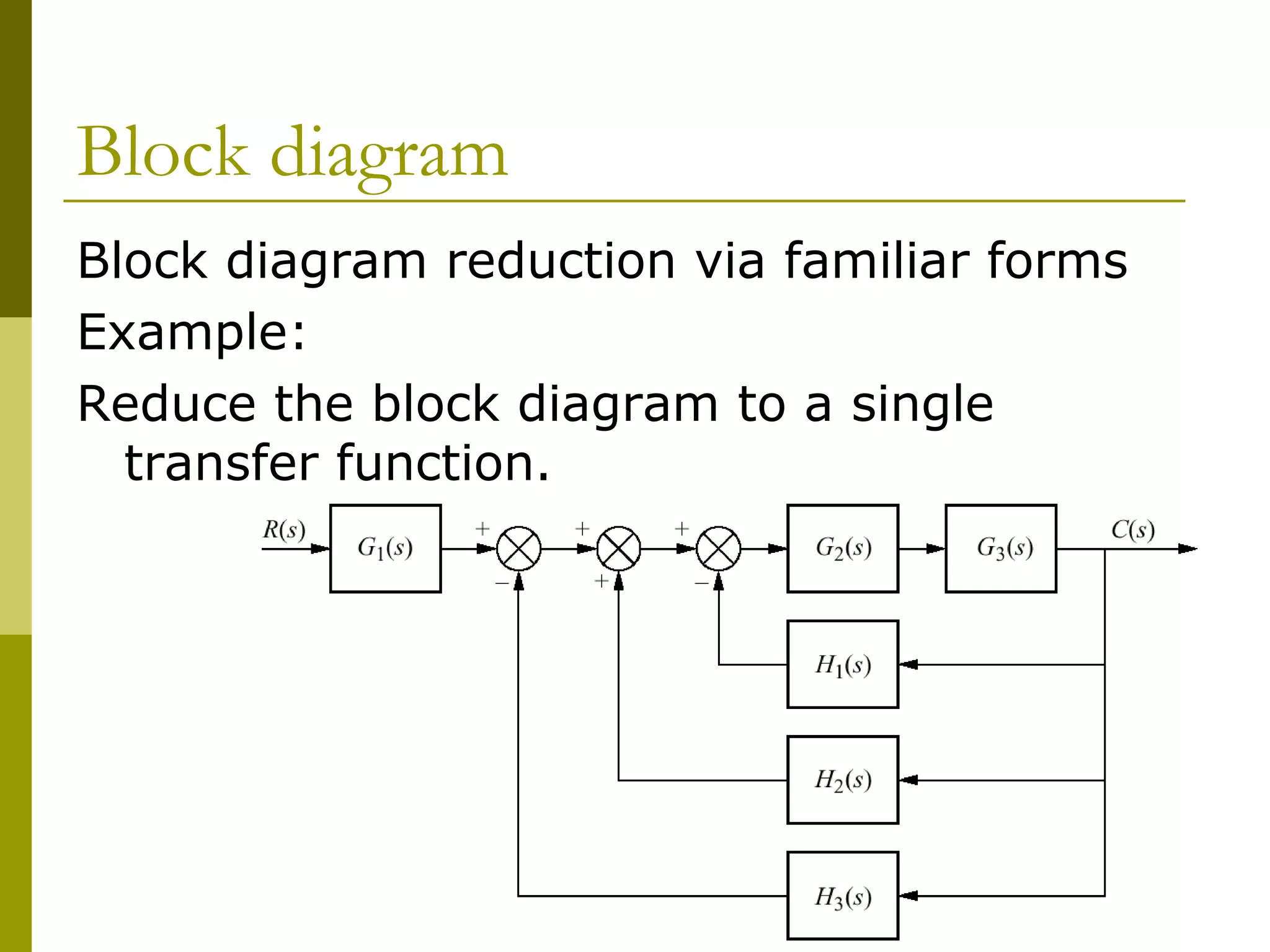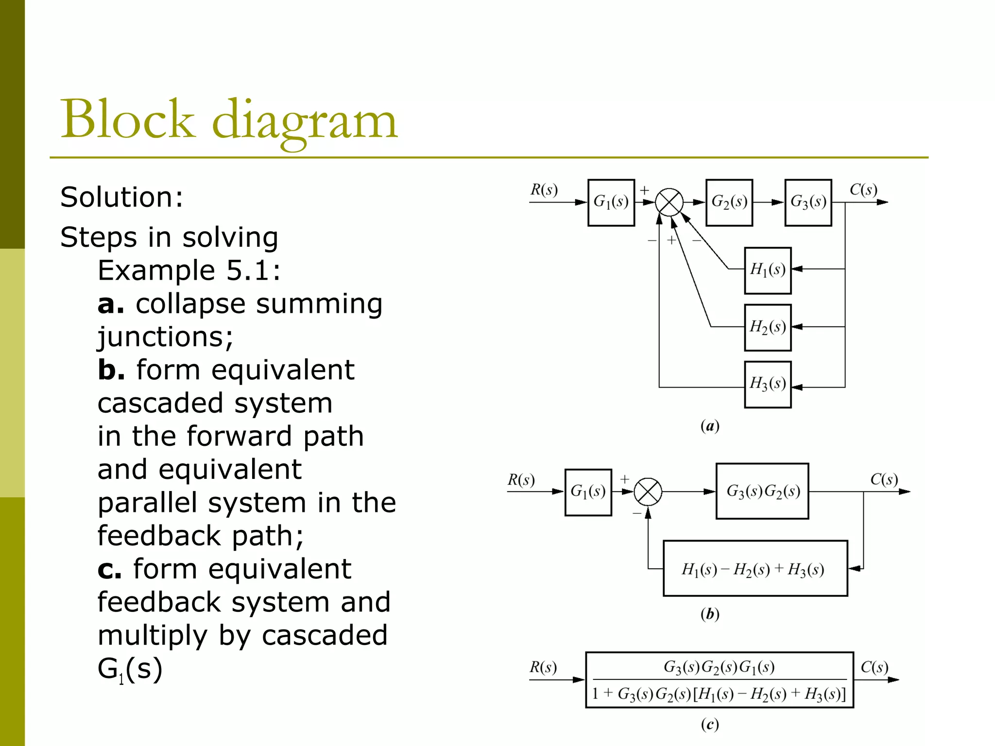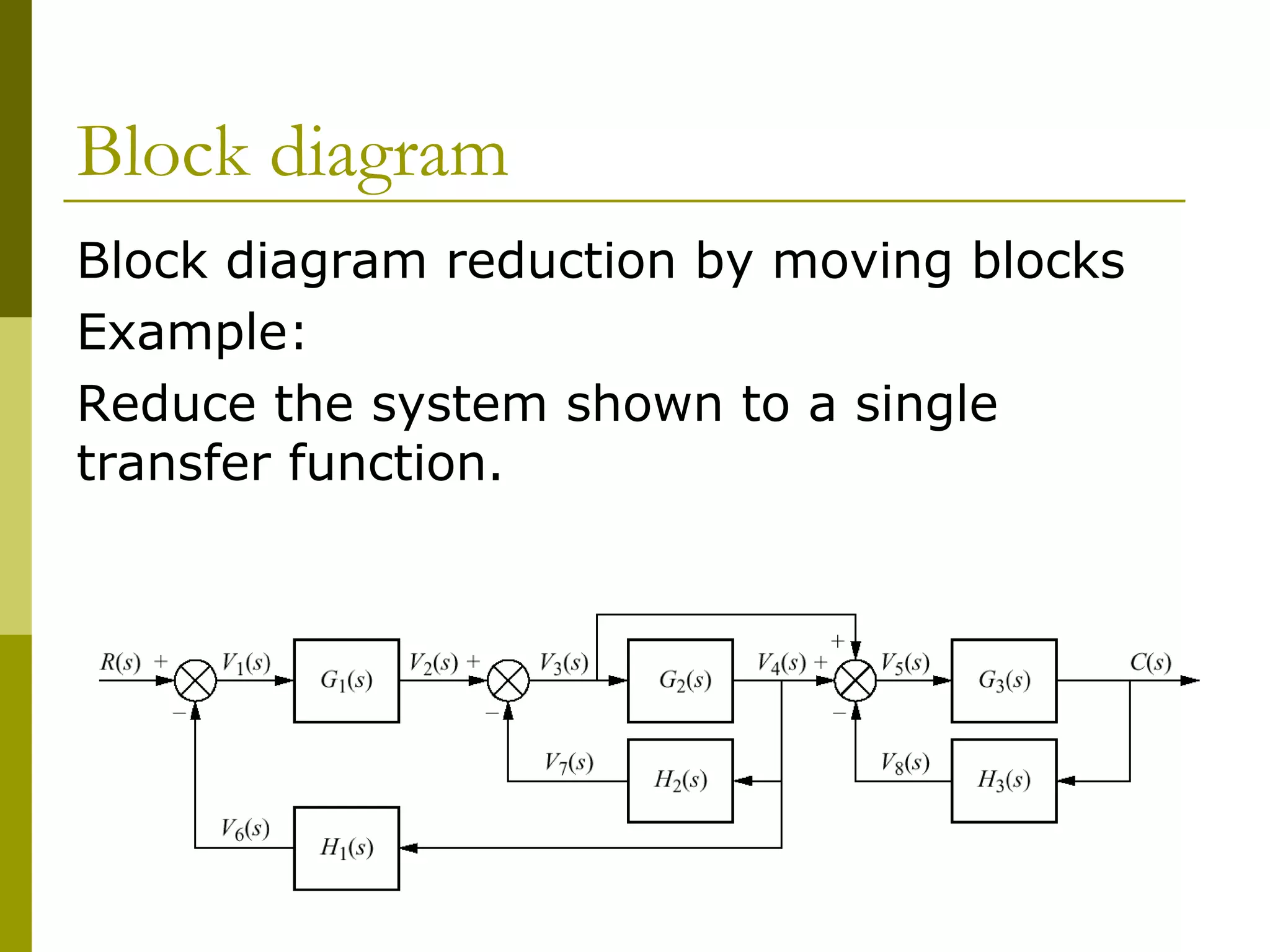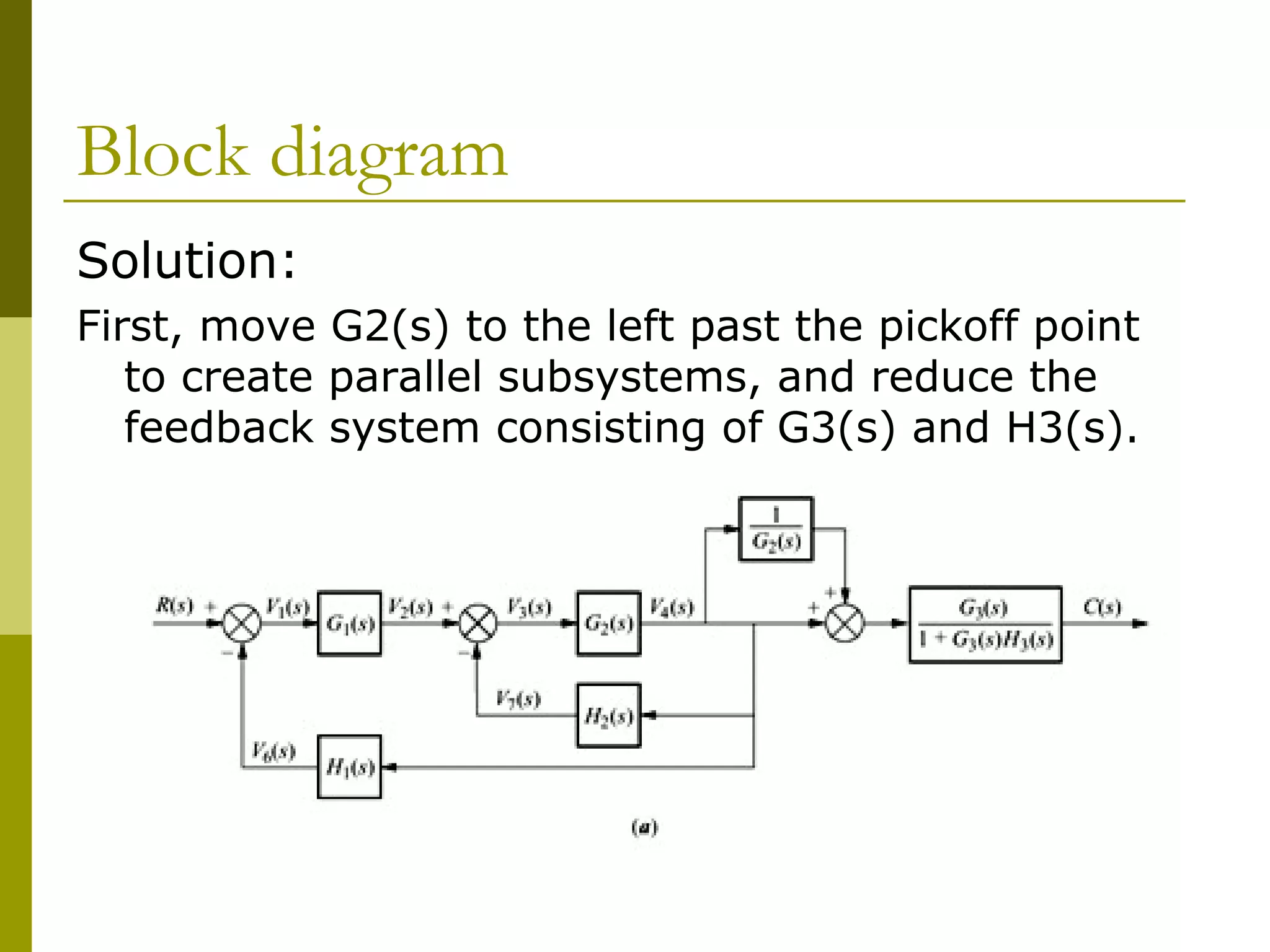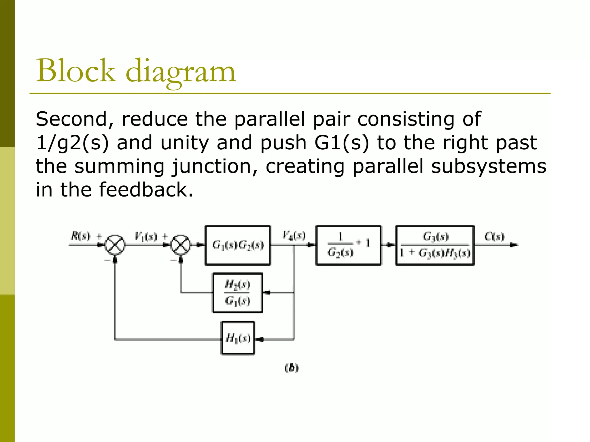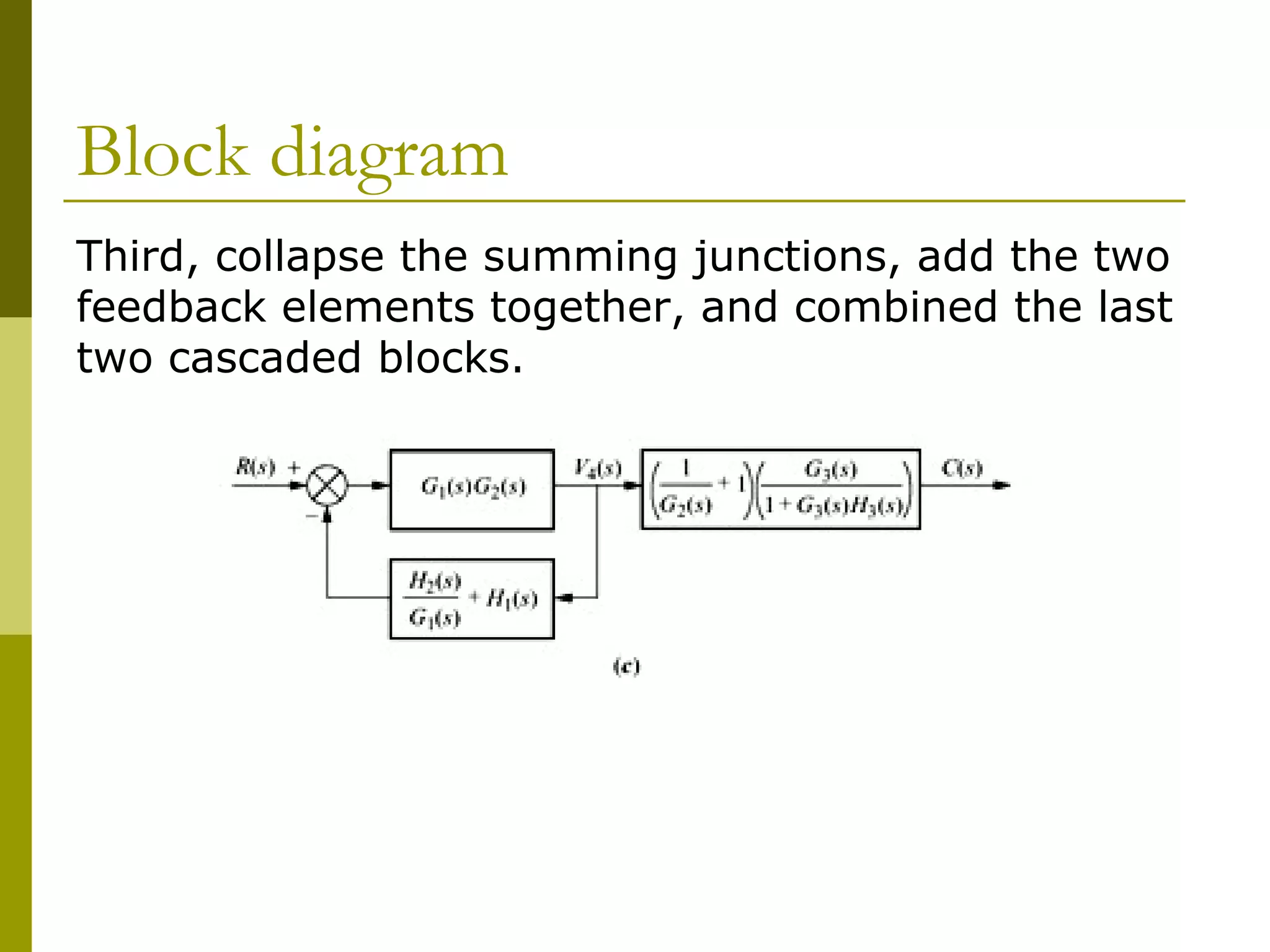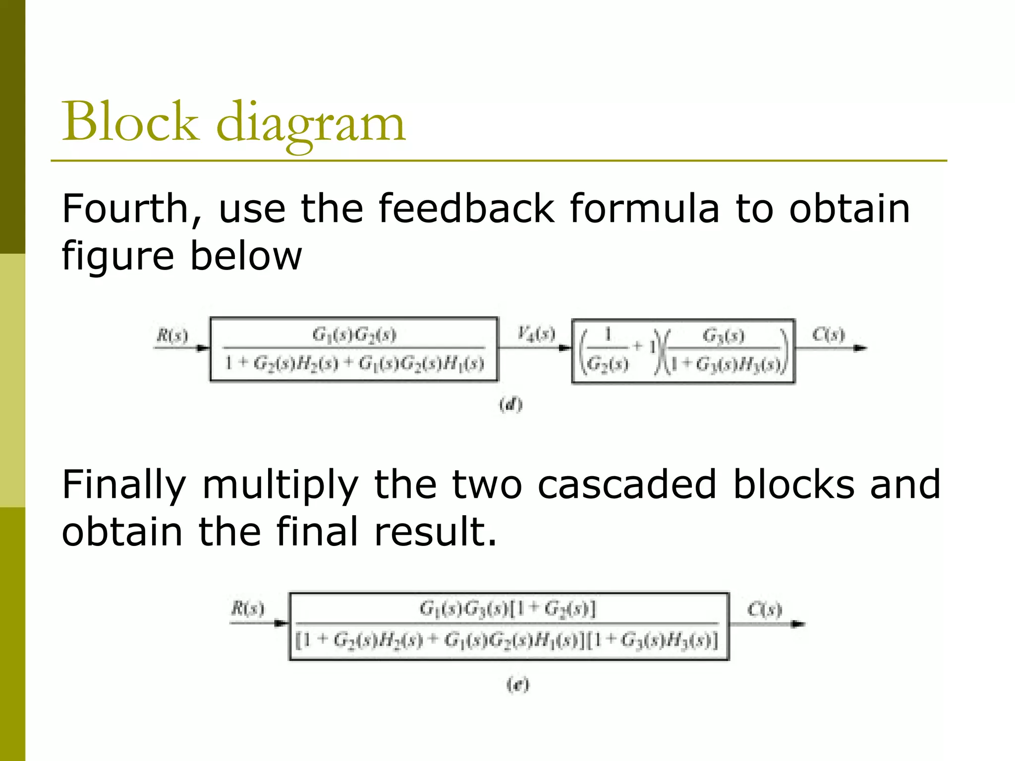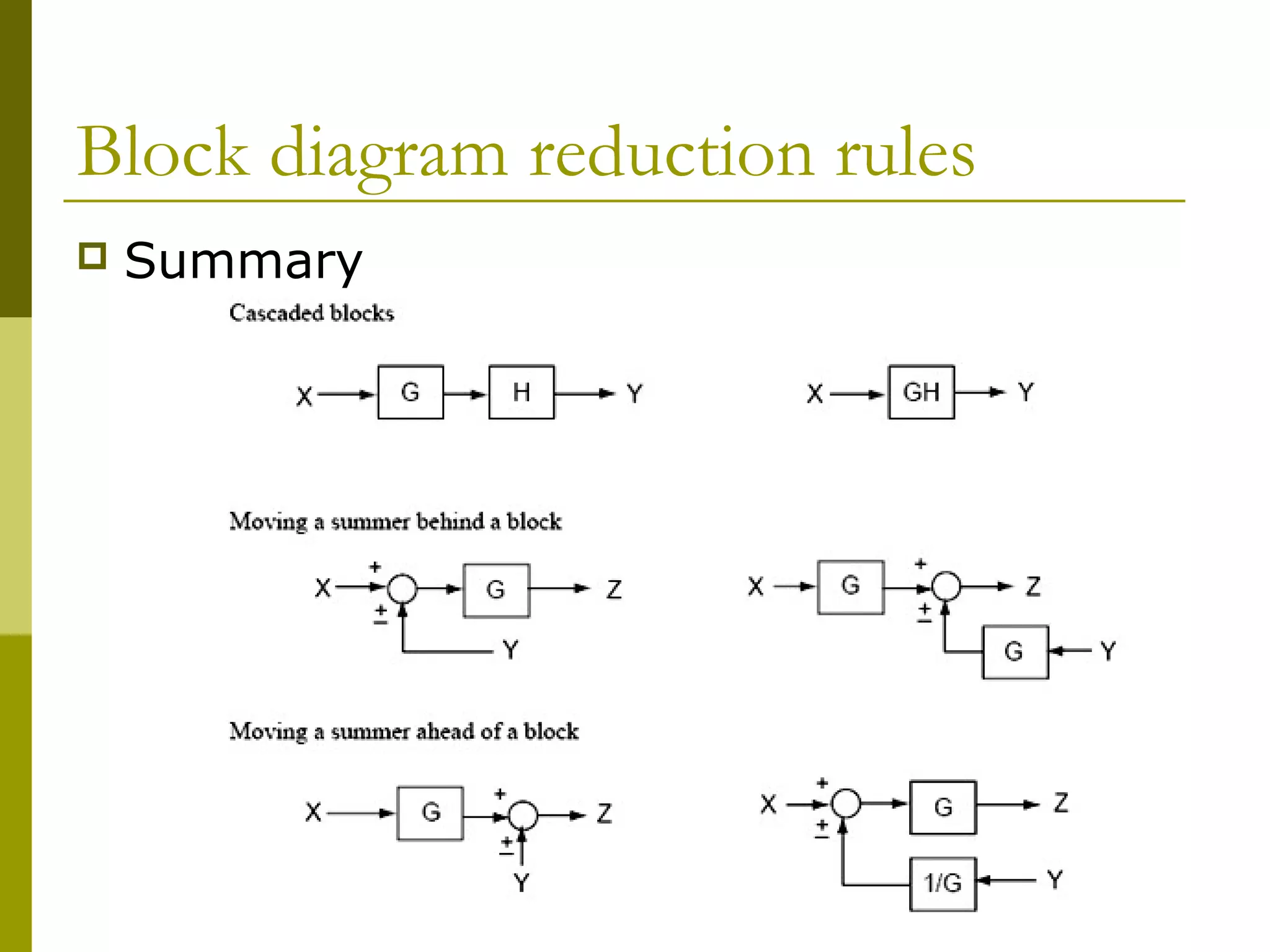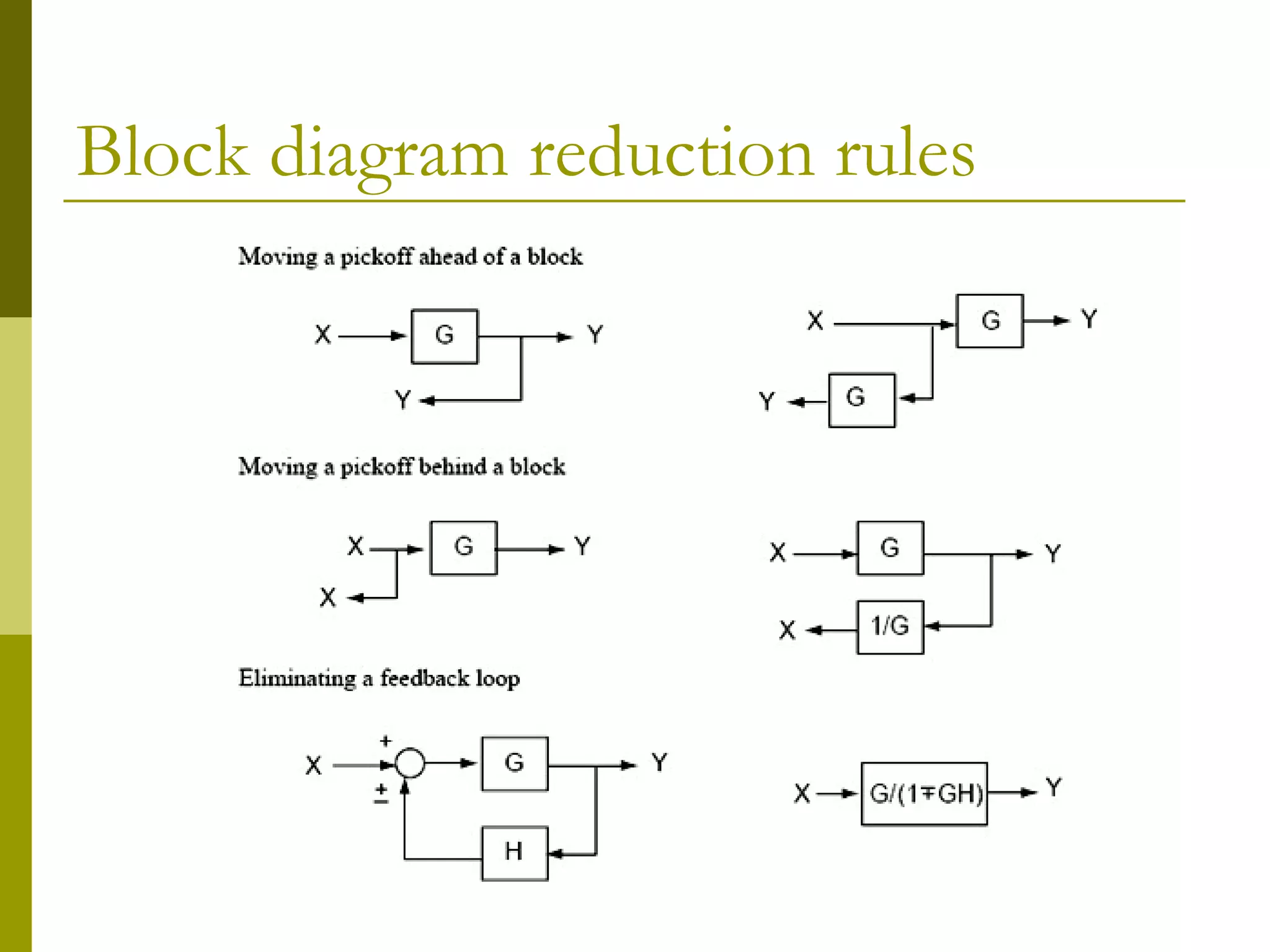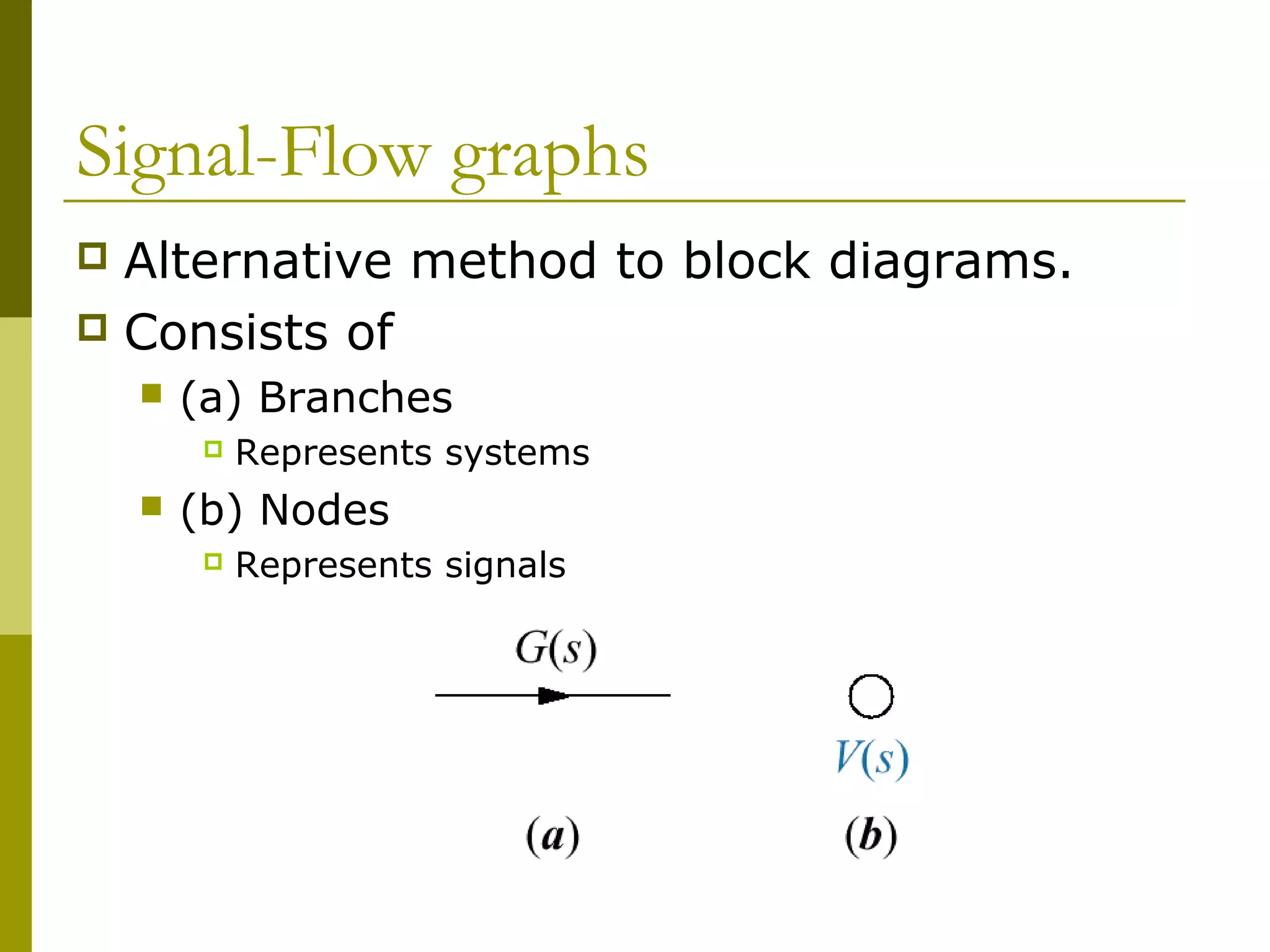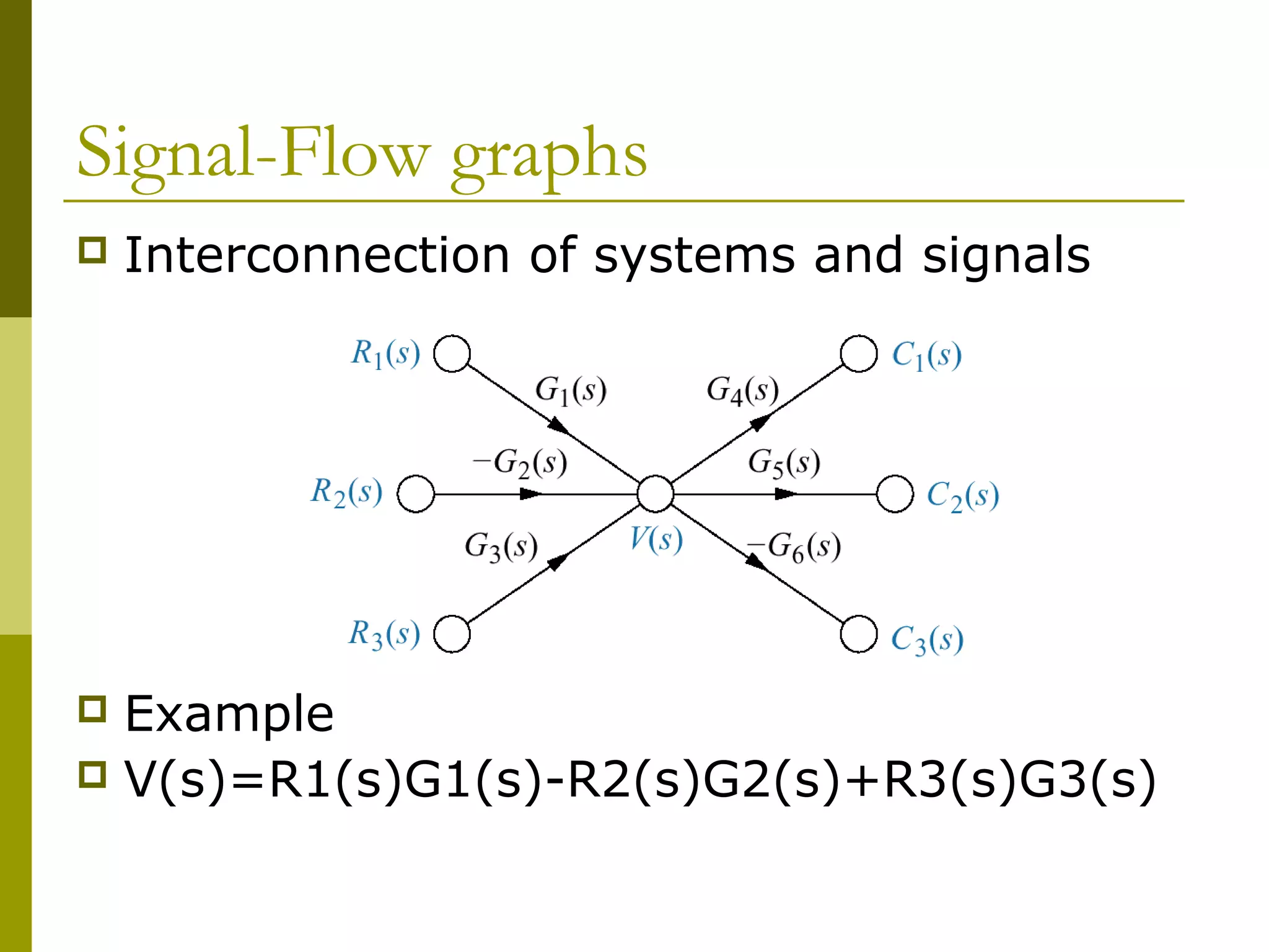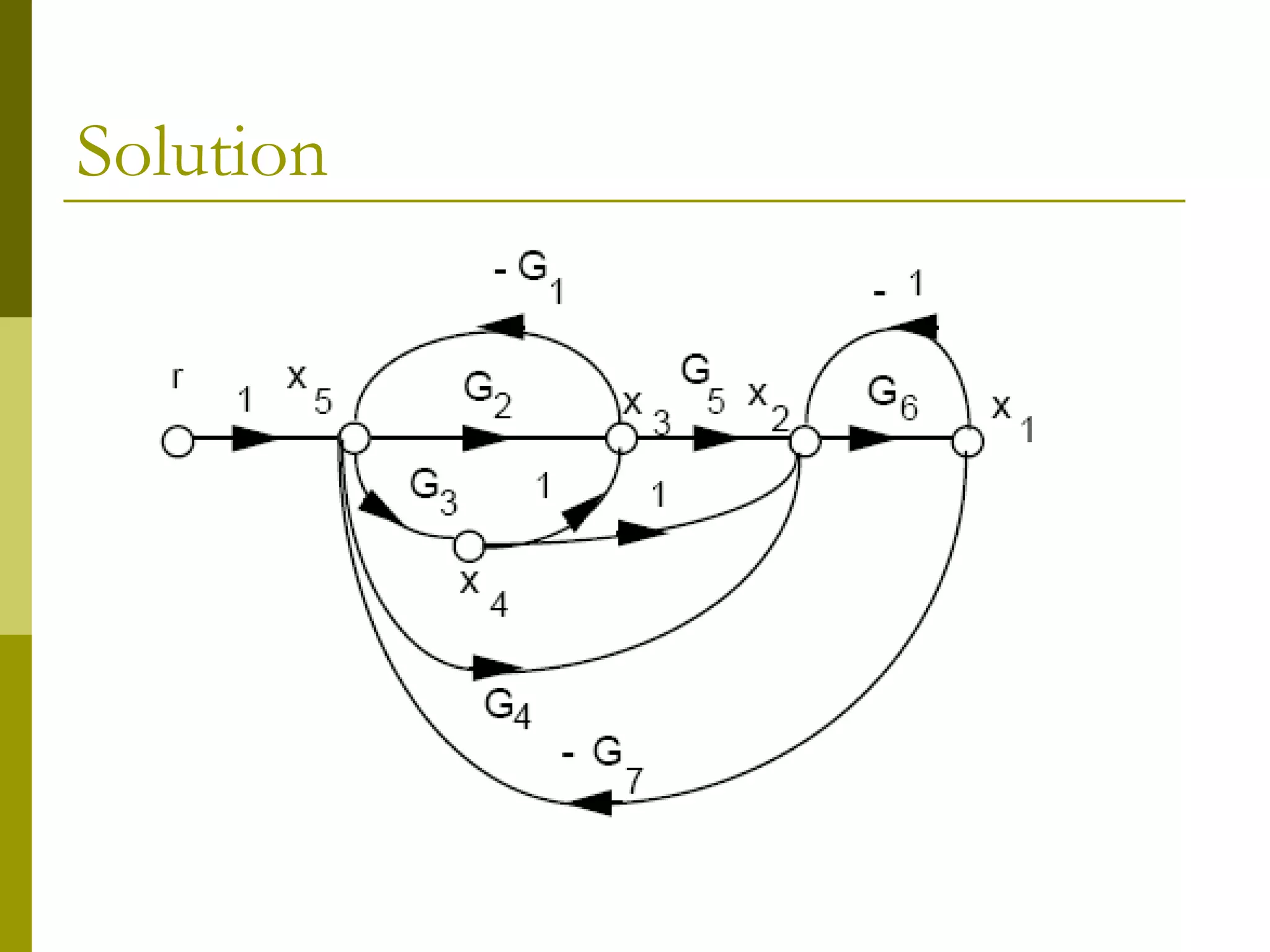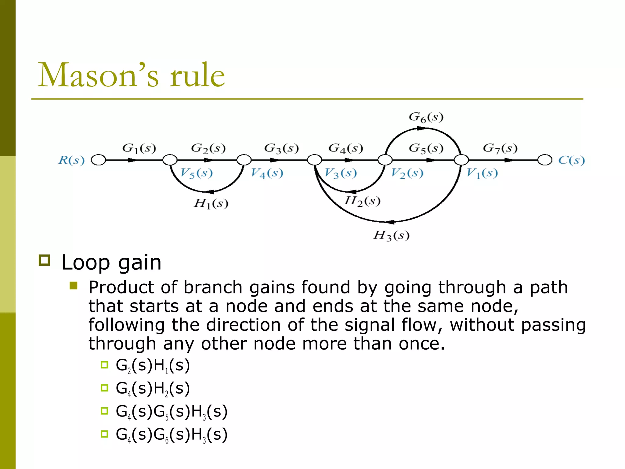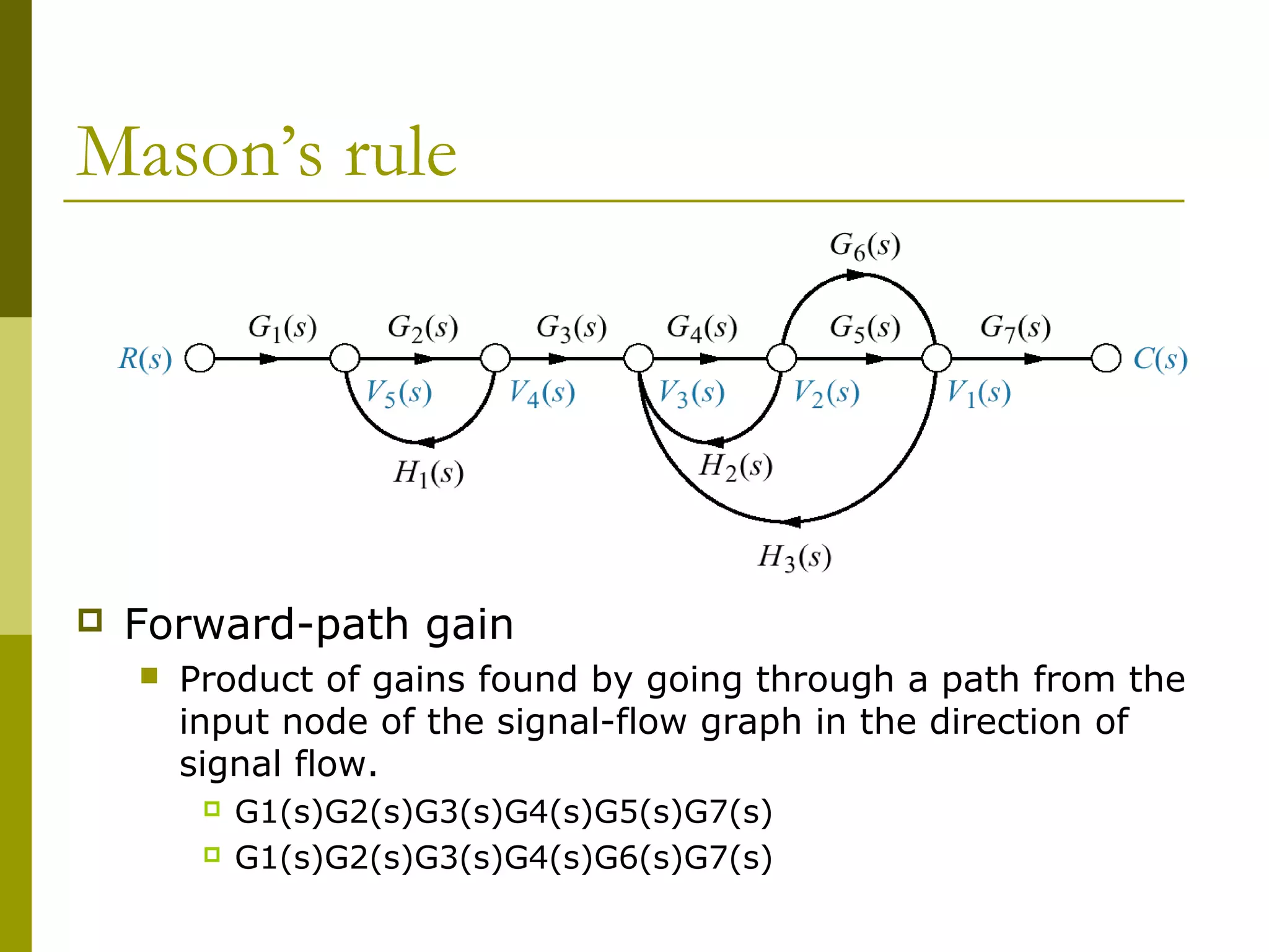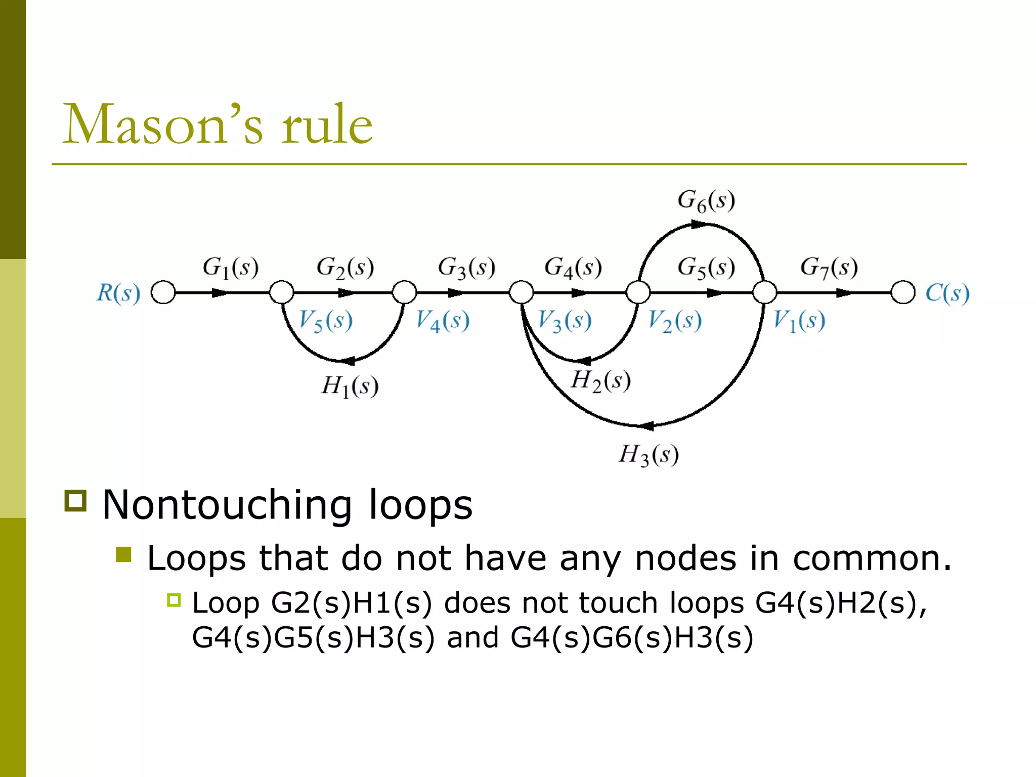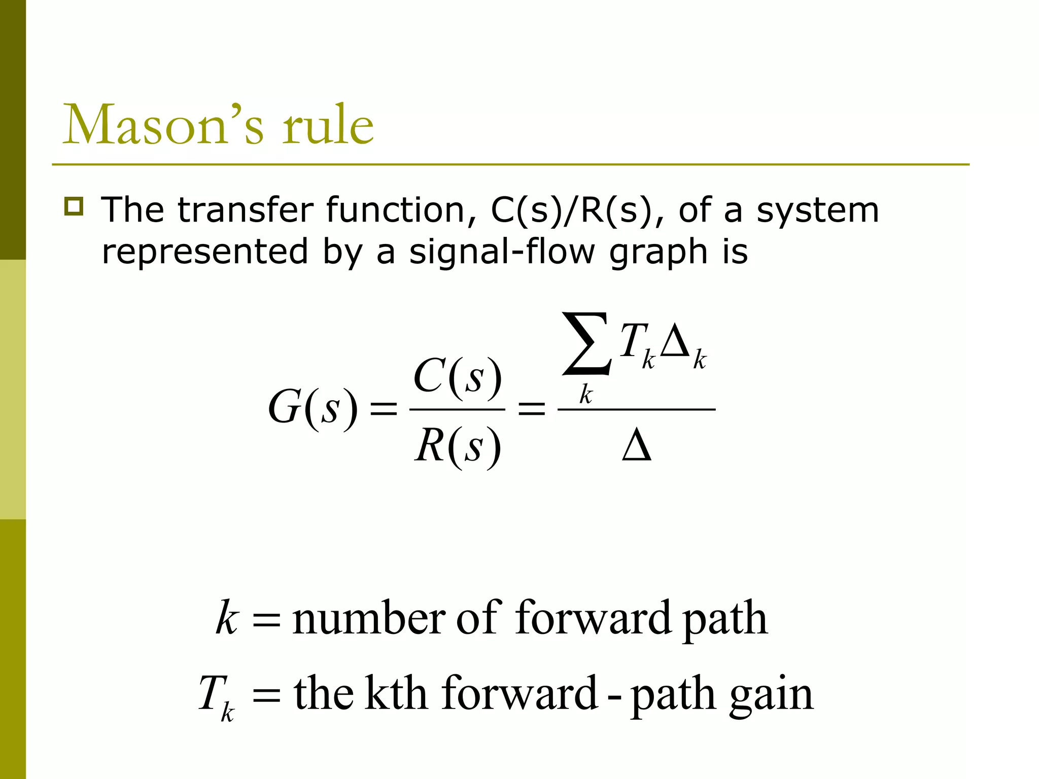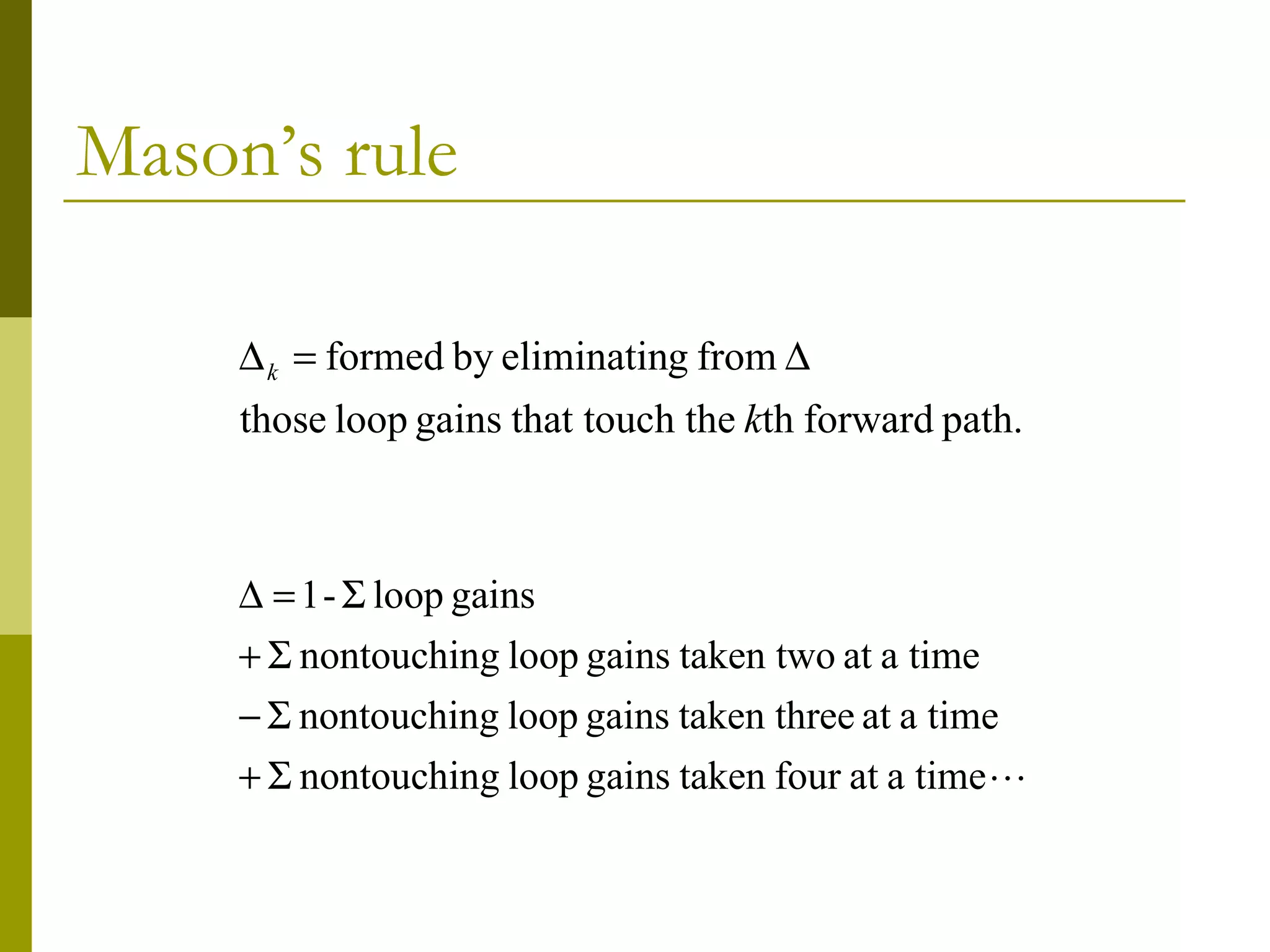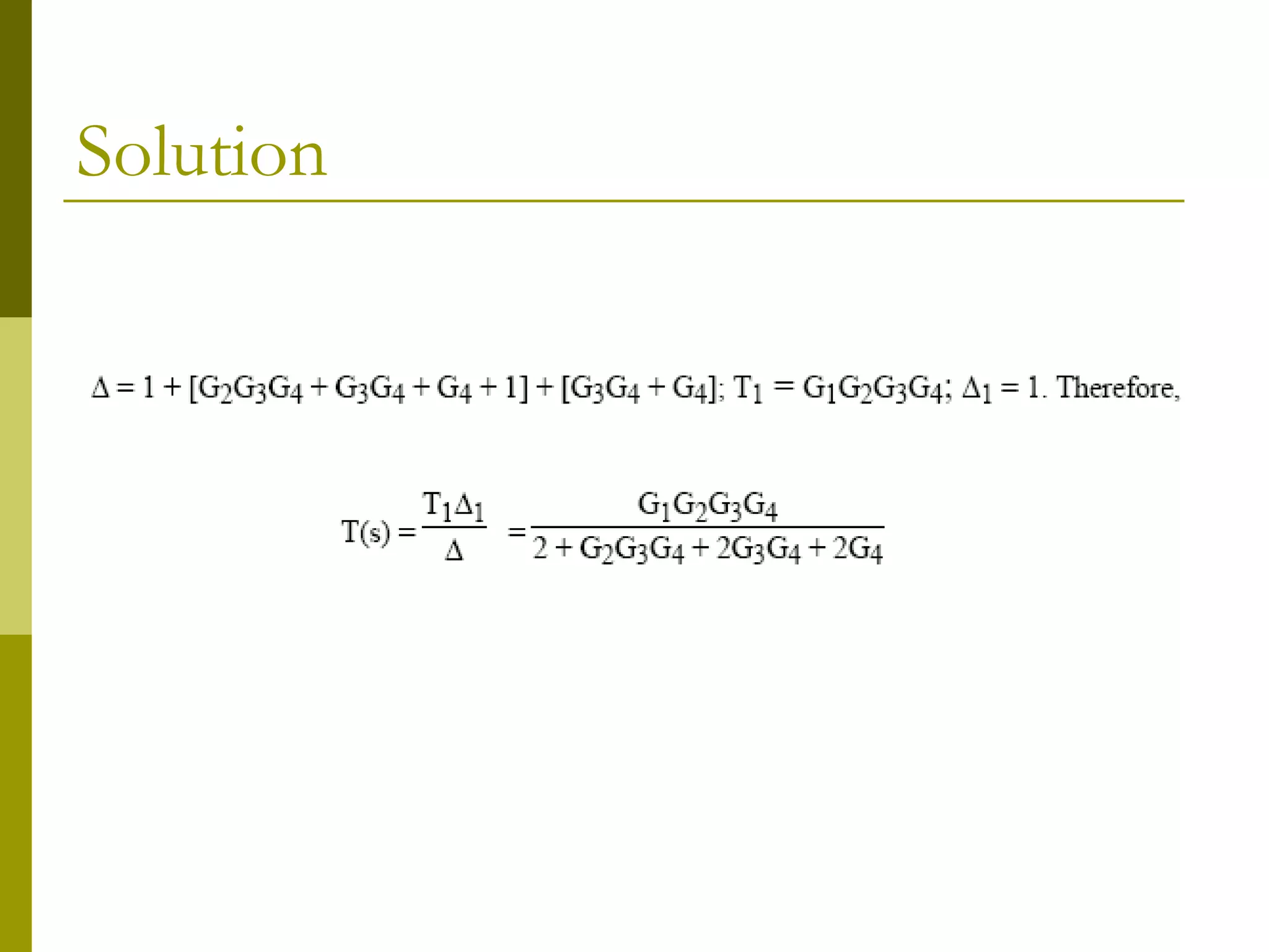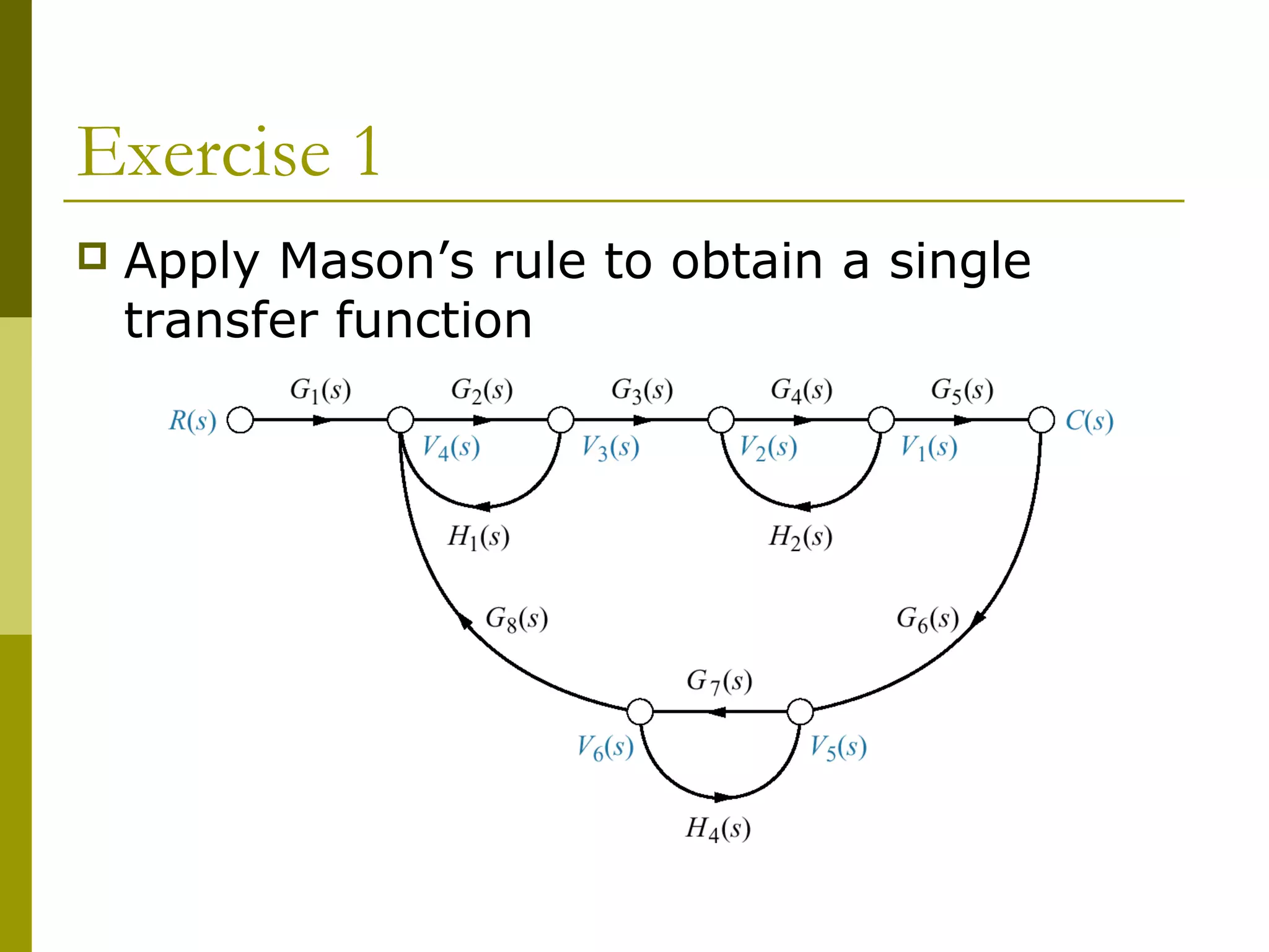The key methods covered are: 1) Representing systems in cascade, parallel, and feedback forms and deriving their equivalent transfer functions 2) Applying algebraic rules to move blocks around diagrams and form familiar topologies 3) Introducing signal flow graphs as an alternative representation 4) Explaining Mason's rule for systematically applying loop and path gains to reduce a signal flow graph down to a single transfer function relating inputs to outputs. 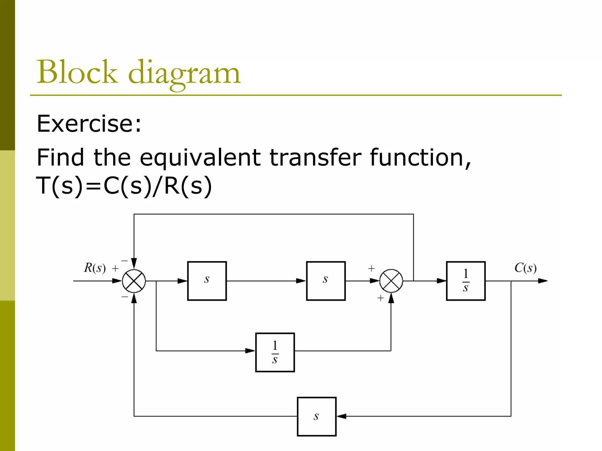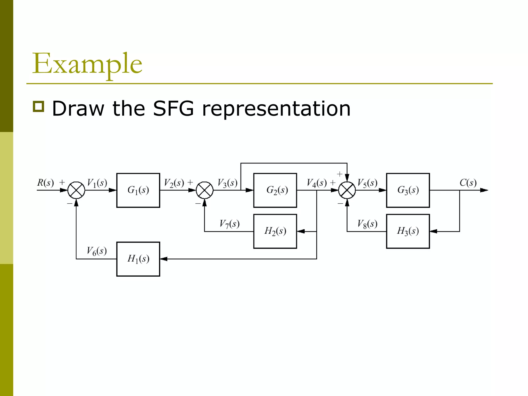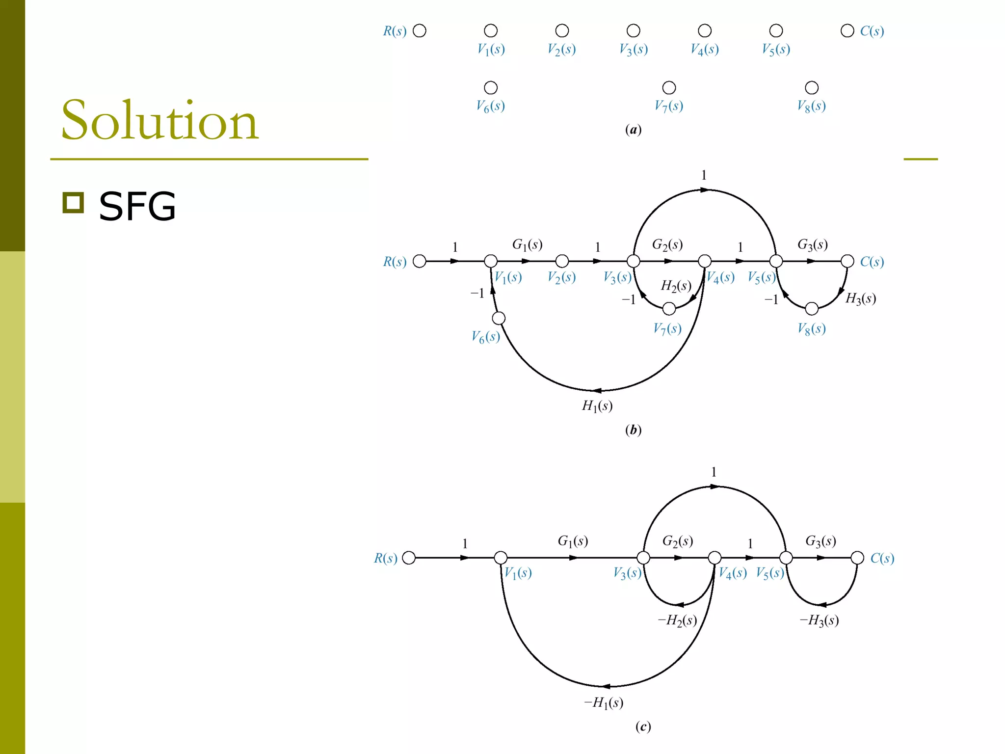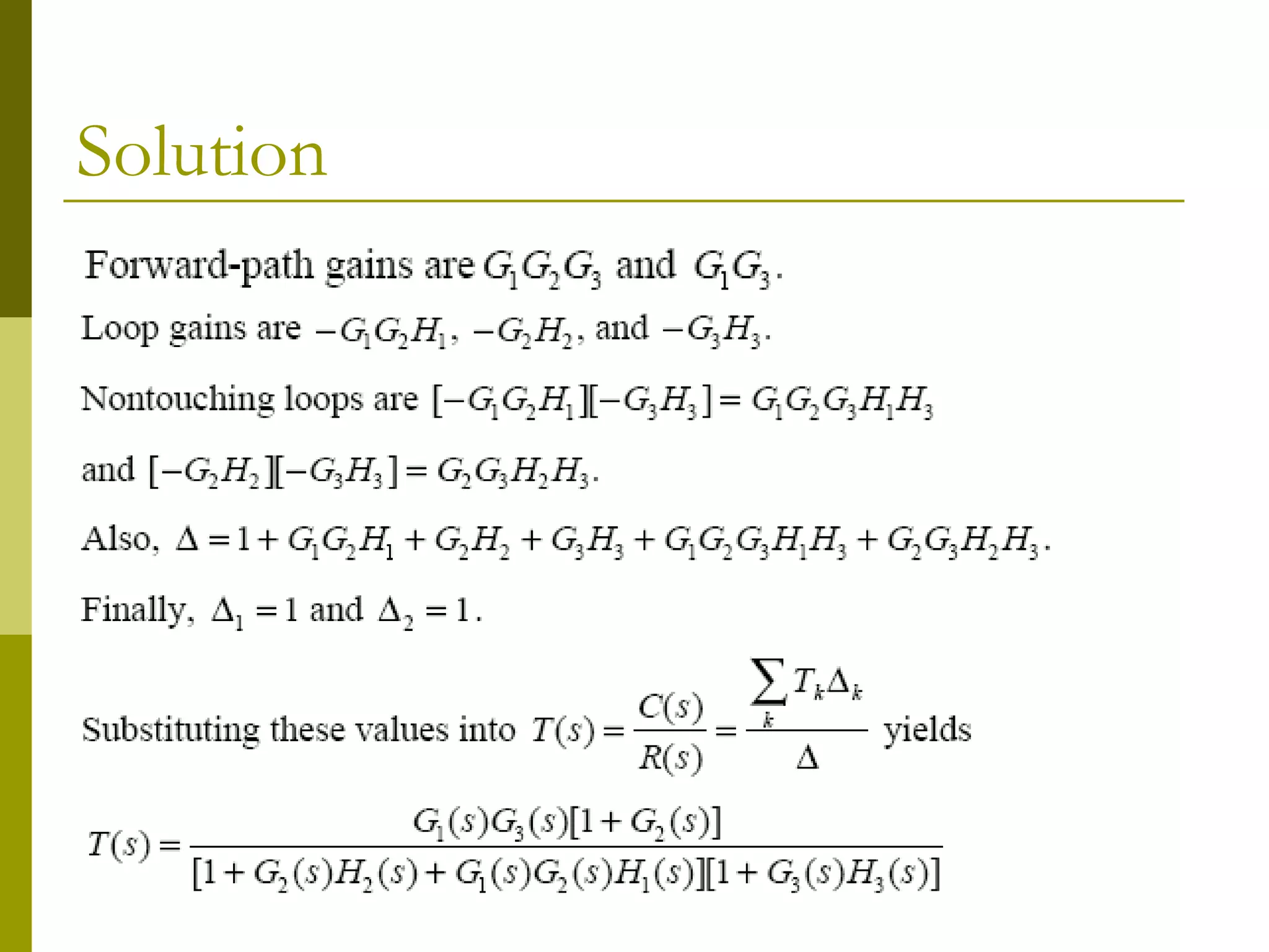Worked examples are provided

1. CONTROL SYSTEMS
THEORY
Reduction of Multiple Subsystems
CHAPTER 3
STB 35103

2. Objectives
 To reduce a block diagram of multiple
subsystems to a signal block representing
the transfer function from input to output

3. Introduction
 Before this we only worked with individual
subsystems represented by a block with
its input and output.
 Complex systems are represented by the
interconnection of many subsystems.
 In order to analyze our system, we want
to represent multiple subsystems as a
single transfer function.

4. Block diagram
 A subsystems is represented as a block
with an input and output and a transfer
function.
 Many systems are composed of multiple
subsystems. So, we need to add a few
more schematic elements to the block
diagram.
 Summing junction
 Pickoff points

5. Block diagram

6. Block diagram
 Summing junction
 Output signal, C(s), is the algebraic sum of the
input signals, R1(s), R2(s) and R3(s).
 Pickoff point
 Distributes the input signals, R(s),
undiminished, to several output points.

7. Block diagram
 There are three topologies that can be
used to reduce a complicated system to a
single block.
 Cascade form
 Parallel form
 Feedback form

8. Block diagram
 Cascade form
 a. cascaded subsystem
 b. equivalent transfer function
 Equivalent transfer function is the output
divided by the input.

9. Block diagram
 Parallel form
 Parallel subsystems have a common input and
output formed by the algebraic sum of the
outputs from all of the subsystems.

10. Block diagram
 Feedback form
 It is the same as the closed loop system that
we learn in Chapter 1.
 a. closed loop system
 b. closed loop, G(s)H(s) is open loop transfer
function

11. Block diagram
 Moving blocks to create familiar forms
 Cascade, parallel and feedback topologies are
not always apparent in a block diagram.
 You will learn block moves that can be made in
order to establish familiar forms when they
almost exist. I.e. move blocks left and right
past summing junctions and pickoff points.

12. Block diagram
Block diagram
algebra for summing
junctions—
equivalent forms for
moving a block
a. to the left past a
summing junction;
b. to the right past a
summing junction

13. Block diagram
Block diagram
algebra for pickoff
points—
equivalent forms
for moving a
block
a. to the left past
a pickoff point;
b. to the right
past a pickoff
point

14. Block diagram
Block diagram reduction via familiar forms
Example:
Reduce the block diagram to a single
transfer function.

15. Block diagram
Solution:
Steps in solving
Example 5.1:
a. collapse summing
junctions;
b. form equivalent
cascaded system
in the forward path
and equivalent
parallel system in the
feedback path;
c. form equivalent
feedback system and
multiply by cascaded
G1(s)

16. Block diagram
Block diagram reduction by moving blocks
Example:
Reduce the system shown to a single
transfer function.

17. Block diagram
Solution:
First, move G2(s) to the left past the pickoff point
to create parallel subsystems, and reduce the
feedback system consisting of G3(s) and H3(s).

18. Block diagram
Second, reduce the parallel pair consisting of
1/g2(s) and unity and push G1(s) to the right past
the summing junction, creating parallel subsystems
in the feedback.

19. Block diagram
Third, collapse the summing junctions, add the two
feedback elements together, and combined the last
two cascaded blocks.

20. Block diagram
Fourth, use the feedback formula to obtain
figure below
Finally multiply the two cascaded blocks and
obtain the final result.

21. Block diagram
Exercise:
Find the equivalent transfer function,
T(s)=C(s)/R(s)

22. Solution
 Combine the parallel blocks in the forward path. Then, push 1/s to
the left past the pickoff point.
 Combine the parallel feedback paths and get 2s. Apply the
feedback formula and simplify

23. Block diagram reduction rules
 Summary

24. Block diagram reduction rules

25. Signal-Flow graphs
 Alternative method to block diagrams.
 Consists of
 (a) Branches
 Represents systems
 (b) Nodes
 Represents signals

26. Signal-Flow graphs
 Interconnection of systems and signals
 Example
 V(s)=R1(s)G1(s)-R2(s)G2(s)+R3(s)G3(s)

27. Signal-Flow graphs
 Cascaded system
Block diagram
Signal flow

28. Signal-Flow graphs
 Parallel system
Block diagram
Signal flow

29. Signal-Flow graphs
 Feedback system
Block diagram
Signal flow

30. SFG
Question
 Given the following block diagram, draw a
signal-flow graph

31. Solution

32. Mason’s rule
 What?
 A technique for reducing signal-flow graphs to
single transfer function that relate the output
of system to its input.
 We must understand some components
before using Mason’s rule
 Loop gain
 Forward-path gain
 Nontouching loops
 Nontouching-loop gain

33. Mason’s rule
 Loop gain
 Product of branch gains found by going through a path
that starts at a node and ends at the same node,
following the direction of the signal flow, without passing
through any other node more than once.
 G2(s)H1(s)
 G4(s)H2(s)
 G4(s)G5(s)H3(s)
 G4(s)G6(s)H3(s)

34. Mason’s rule
 Forward-path gain
 Product of gains found by going through a path from the
input node of the signal-flow graph in the direction of
signal flow.
 G1(s)G2(s)G3(s)G4(s)G5(s)G7(s)
 G1(s)G2(s)G3(s)G4(s)G6(s)G7(s)

35. Mason’s rule
 Nontouching loops
 Loops that do not have any nodes in common.
 Loop G2(s)H1(s) does not touch loops G4(s)H2(s),
G4(s)G5(s)H3(s) and G4(s)G6(s)H3(s)

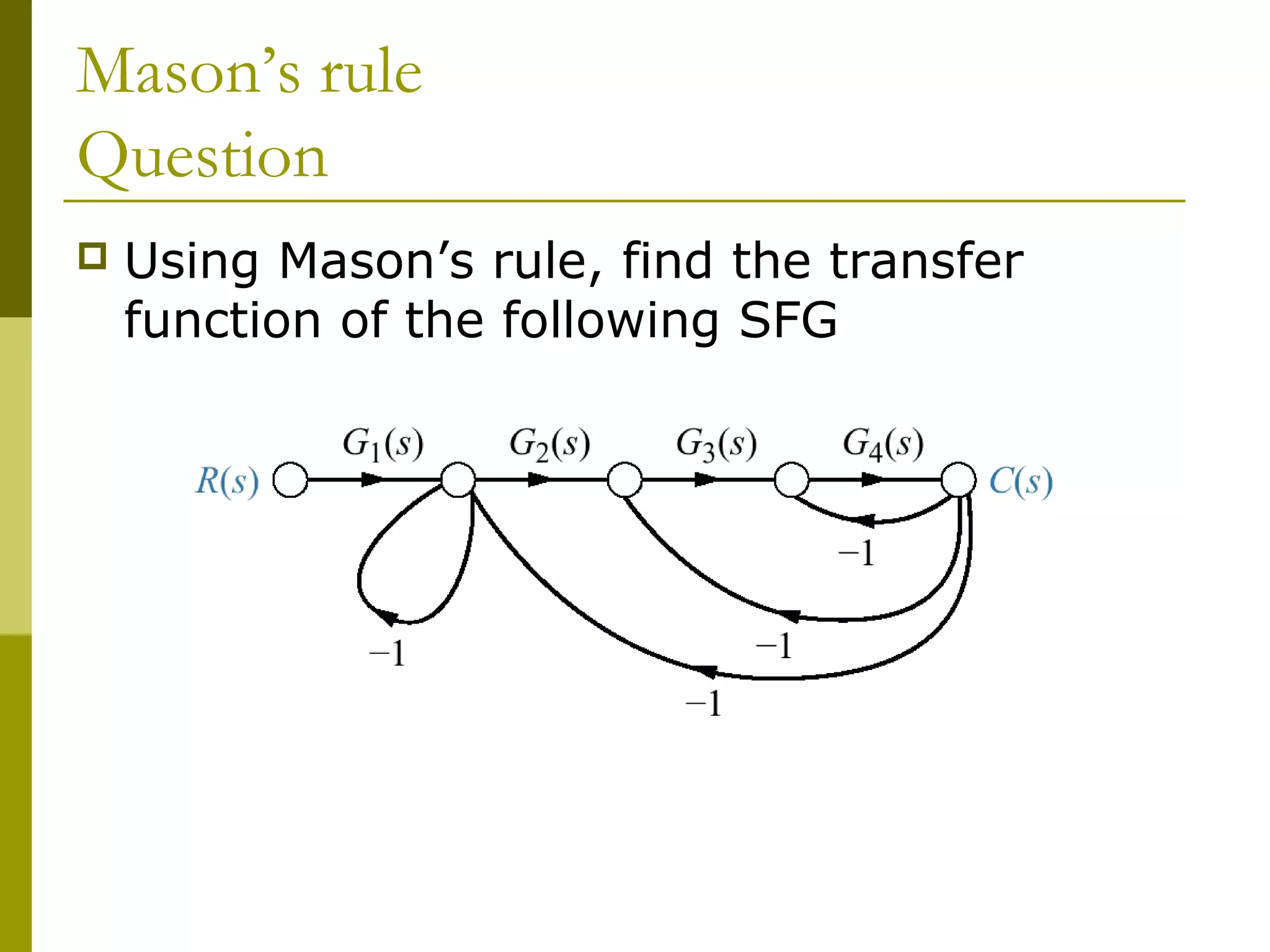
36. Mason’s rule
 Nontouching-loop gain
 Product of gains form nontouching loops taken
two, three, four, or more at a time.
 [G2(s)H1(s)][G4(s)H2(s)]
 [G2(s)H1(s)][G4(s)G5(s)H3(s)]
 [G2(s)H1(s)][G4(s)G6(s)H3(s)]

37. Mason’s rule
 The transfer function, C(s)/R(s), of a system
represented by a signal-flow graph is
∆
∆
=
=
∑
k
k
k
T
s
R
s
C
s
G
)
(
)
(
)
(
gain
path
-
forward
kth
the
path
forward
of
number
=
=
k
T
k

38. Mason’s rule

time
a
at
four
taken
gains
loop
g
nontouchin
time
a
at
ee
taken thr
gains
loop
g
nontouchin
time
a
at
taken two
gains
loop
g
nontouchin
gains
loop
-
1
Σ
+
Σ
−
Σ
+
Σ
=
∆
path.
forward
th
h the
that touc
gains
loop
those
from
g
eliminatin
by
formed
k
k ∆
=
∆

39. Example
 Draw the SFG representation

40. Solution
 SFG

41. Solution

42. Mason’s rule
Question
 Using Mason’s rule, find the transfer
function of the following SFG

43. Solution

44. Exercise 1
 Apply Mason’s rule to obtain a single
transfer function

45. Exercise 2
1. Reduce to a single transfer function (BDR)
2. Draw the SFG representation
3. Apply Mason’s rule to obtain the transfer function