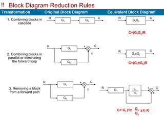
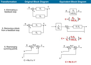
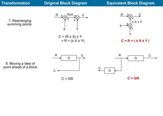
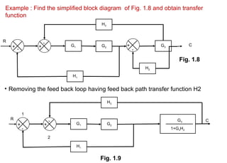
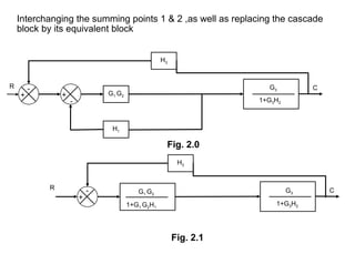
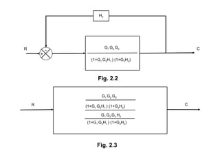
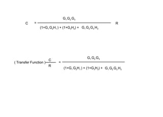
The document explains control systems, defining control as the regulation of a system to achieve objectives. It covers components like inputs, outputs, block diagrams, transfer functions, and their properties, advantages, and disadvantages, while emphasizing their role in linear systems. Additionally, it discusses multi-loop control and block diagram reduction rules for simplification.

1. ‼ Control
• The meaning of control is to regulate, direct or command a system so that
a desire objective is obtained.
‼ Control system
• It is an amalgamation of different physical elements linked in such a
manner so as to regulate, direct or command itself to obtain certain
objectives.
or
• Control system is a science, which deals with mechanisms, devices or
objects joined together for the interaction with the aim to achieve the
desired results.

2. Input: The applied signal or excitation signal that is applied to control system
to get a specified output is called input
Output: The actual response that is obtained from a control system due to
the application of the input is termed as Output
Fig. 1 Cause and effect relationship between the input and output
Control ActionInput Output
A control system must have
• Input
• Output
• Way to achieve input and output objectives
• Control action

3. ‼ Block Diagram
• The shorthand pictorial representation of the cause-and –effect relationship
between the input and output of a physical system is known as block
diagram.
Input
G(s) C(s)R(s)
OutputBlock
Fig. 1.1 A simple Block
Fig. 1.62 Block Diagram with gain

4. ‼ Definition of basic elements of the block diagram
• Summing point : Its is a small circle with appropriate plus and minus sign
associated with the arrows entering the circle. The output is the algebraic
sum of the inputs. There is no limit on the number of inputs entering a
summing point.
+
+
+
-
+
X(s) X(s) C(s)
Z(s)
C(s)
Y(s)
Y(s)
Fig. 1.3 Summer with Two
Inputs
Fig. 1.4 Summer with Three
Inputs

5. X(s) and Y(s) are inputs while C(s) is
output.
C(s) = X(s) + Y(s)
C(s)
X(s) ,Y(s) and Z(s) are inputs while C(s)
is output.
C(s) = X(s) -Y(s) + Z(s)
+
+
X(s) C(s)
Y(s)
Fig. 1.3 Summer with Two Inputs
+
-
+
X(s)
Z(s)
Y(s)
Fig. 1.4 Summer with Three Inputs

6. • Take off Point : A take off point allows the same signal or variable as input
to more than one block or summing point, thus permitting the signal to
proceed unaltered along several different paths to several destinations.
X(s)
X(s)
X(s)
X(s)
Take off point
Fig. 1.5 Take off point

7. • Forward Path : The direction of flow of signal from input to output is
known as forward path.
• Feedback Path: The direction of flow of signal from input to output is
known as forward path.
G1(s) G3(s)G2(s)
Input Output
Fig. 1.6 Forward Path
Fig. 1.6 Forward Path
G1(s) G2(s)
H(s)
+
-

8. ‼ Transfer Function
Transfer Function : It is the ratio of the Laplace transform of output
to the Laplace transform of input (excitation) assuming all the initial
conditions to be zero.
If G(s) be the transfer function of the system, we can write
mathematically
G(s) = Laplace transform of output
Laplace transform of input all initial conditions are zero
C(s)R(s) G(s)
C(s)
R(s) all initial conditions are zero

9. ‼ Properties of Transfer function (TF)
• The ratio of Laplace transform of output to input will all initial conditions to be
zero is known as transfer function of a system.
• Transfer function cannot be defined for non-linear systems.it can be defined
for linear systems only.
• The system poles and zeroes can be determined from its characteristic
equitation.
• The transfer function of a system does not depend on the inputs to the
system.
• Stability can be found from characteristic equation.

10. ‼ Advantages of transfer function :
• Transfer function is a mathematical model and it gives the gain of the
system
• Since Laplace transform is used, the terms are simple algebraic
expressions and differential terms are not present.
• If transfer function of a system in known, the response of the system to any
input can be determined very easily.
• Transfer function helps in the study of stability analysis of the system.
• Poles and zeroes of a system can be determined from the knowledge of the
transfer function of he system. Both poles and zeros have a vital role in the
system’s response.

11. ‼ Disadvantages of transfer function :
• Transfer function can be defined for linear systems only.
• Initial conditions lose their importance since transfer function does not take
into account the initial condition
• No inferences can be drawn about the physical structure of a system from
its transfer function.

12. ‼ Laplace Transform
• The Method of transforming a function from time domain into s domain is
known as Laplace transform, where s is a complex operator denoted by
s = ϭ + ωϳ
In other words, the Laplace transform will change a function in time domain to
s domain.
Multi loop control system
•Multiple loop control means you use multiple feedbacks in a cascade form to
influence your controlling medium. This is more rare and is only required in
specific situations

13. Transformation Original Block Diagram Equivalent Block Diagram
G1 G2
R C
G1G2
R C
C=(G1G2)R
1. Combining blocks in
cascade
2. Combining blocks in
parallel or eliminating
the forward loop
G1±G2
R
C=(G1±G2)R
3. Removing a block
from a forward path
G1
G2
±
+ CR
G1
G2
±
+ CR
G1
R
G2
G1
C
C
±
+
C= G2 (1±
G2
G1 ±1) R
‼ Block Diagram Reduction Rules

14. Transformation Original Block Diagram Equivalent Block Diagram
G1
G2
R
±
C
1±G1G2
G2R C
G2
1±G1G2
( )C = R
4. Eliminating a
feedback loop
5. Removing a block
from a feedback loop
1
G2
G1 G2
±
+
1
G2
G1G2
1±G1G2
)(C = R
G1
G2
R
±
C
6. Rearranging
summing points
C = R± X ± Y
±
R R±Y ++ C
Y
X
±
±
R R±X ++ C
X
Y
±
C = R± X ± Y

15. Transformation Original Block Diagram Equivalent Block Diagram
C = (R ± X) ± Y
= R + (± X ± Y)
Y
C = R + ( ± X ± Y )
±
R
± X ± Y
+ C
+
±
X
X Y
±
R R±X ++ C
±7. Rearranging
summing points
G
R C
C
C = GR
G
G
C
CR
C = GR
8. Moving a take of
point ahead of a block

16. G1 G2
G3
H3
H1
H2
+
-
-
+
-
+
• Removing the feed back loop having feed back path transfer function H2
Example : Find the simplified block diagram of Fig. 1.8 and obtain transfer
function
Fig. 1.8
Fig. 1.9
C
C
R
G3
1+G3H2
G1 G2
H3
H1
+
-
-
+
R
1
2

17. Interchanging the summing points 1 & 2 ,as well as replacing the cascade
block by its equivalent block
G1 G2
H3
H1
+
-
-
+
R G3
1+G3H2
C
Fig. 2.0
H3
-
+
CG3
1+G3H2
G1 G2
1+G1 G2H1
R
Fig. 2.1

18. C
H3
-
+
G1 G2 G3
(1+G1 G2H1 ) (1+G3H2)
R
G1 G2 G3
(1+G1 G2H1 ) (1+G3H2)
G1 G2 G3 H3
(1+G1 G2H1 ) (1+G3H2)
R C
Fig. 2.2
Fig. 2.3

19. G1 G2 G3
(1+G1 G2H1 ) + (1+G3H2) + G1 G2 G3 H3
C R=
C
R
G1 G2 G3
(1+G1 G2H1 ) + (1+G3H2) + G1 G2 G3 H3
=( Transfer Function )