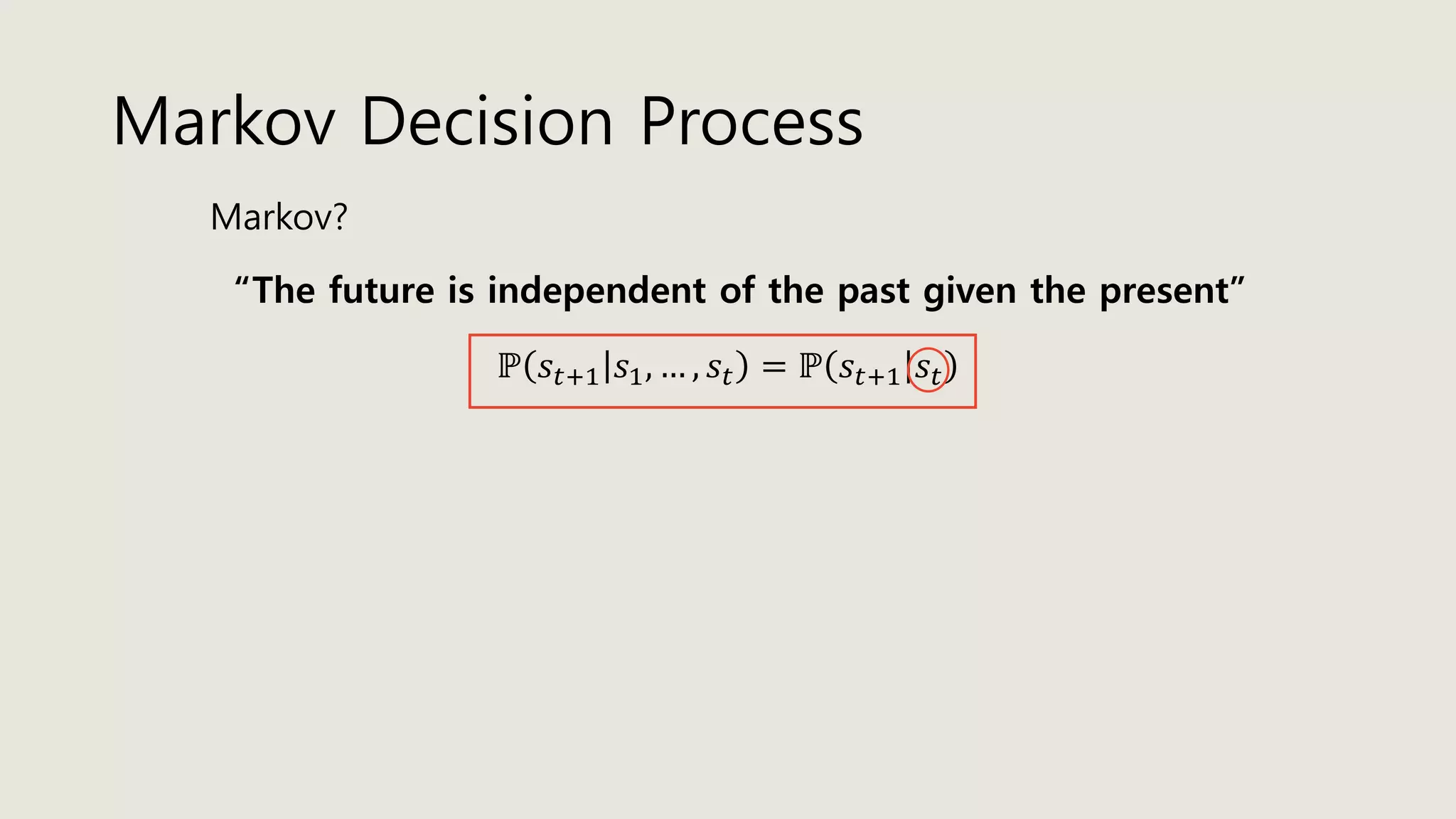
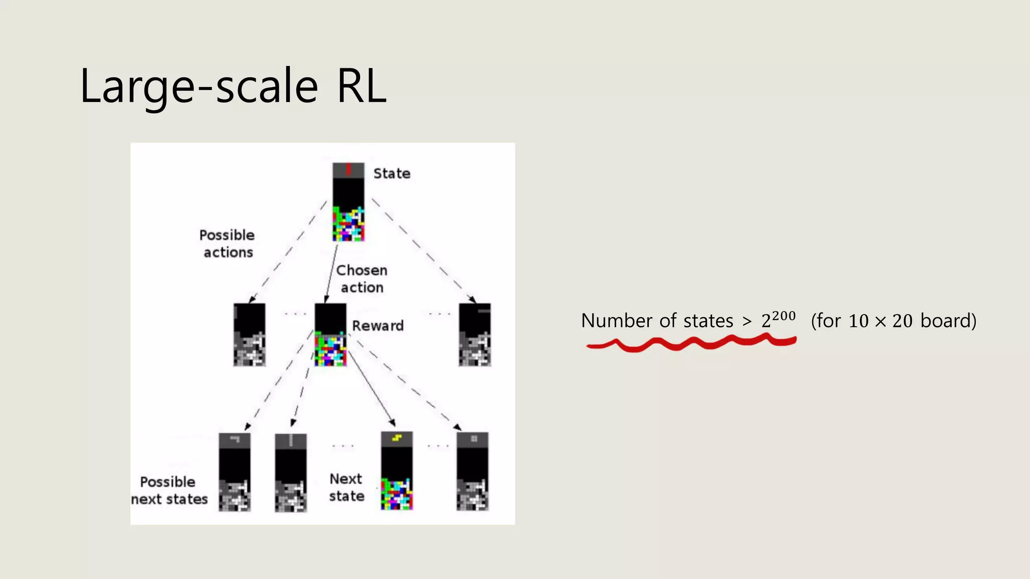
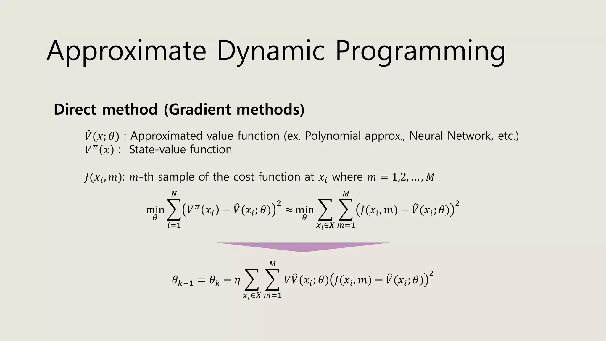
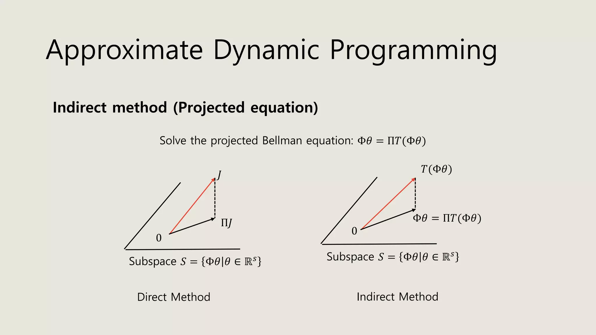
The document discusses stochastic optimal control and reinforcement learning (RL), detailing concepts such as Markov decision processes, policies, value functions, and various algorithms for optimizing control. Key topics include reinforcement learning terminology, Bellman operators, and dynamic programming techniques used to solve control problems in both infinite and finite horizons. The document also explores model-based and model-free approaches to estimating dynamics and rewards in RL.


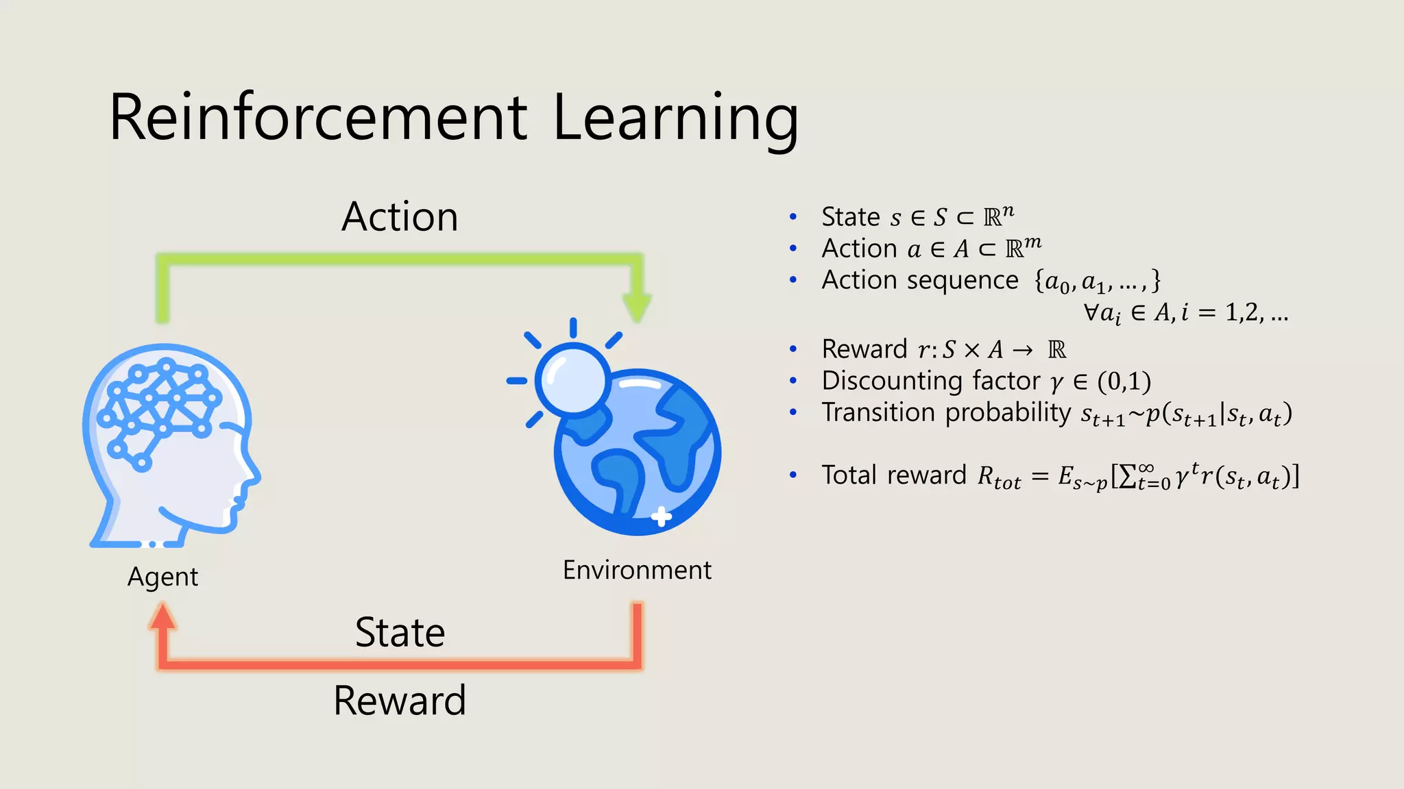

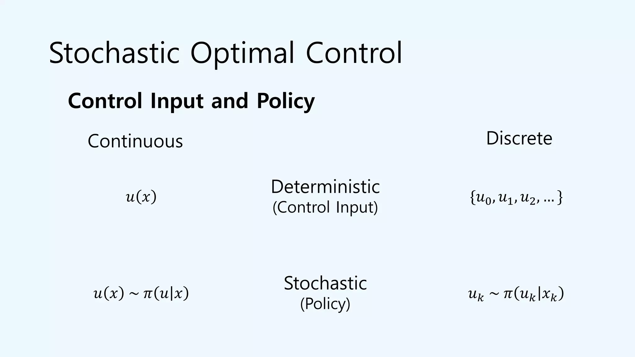
![Bellman Operator
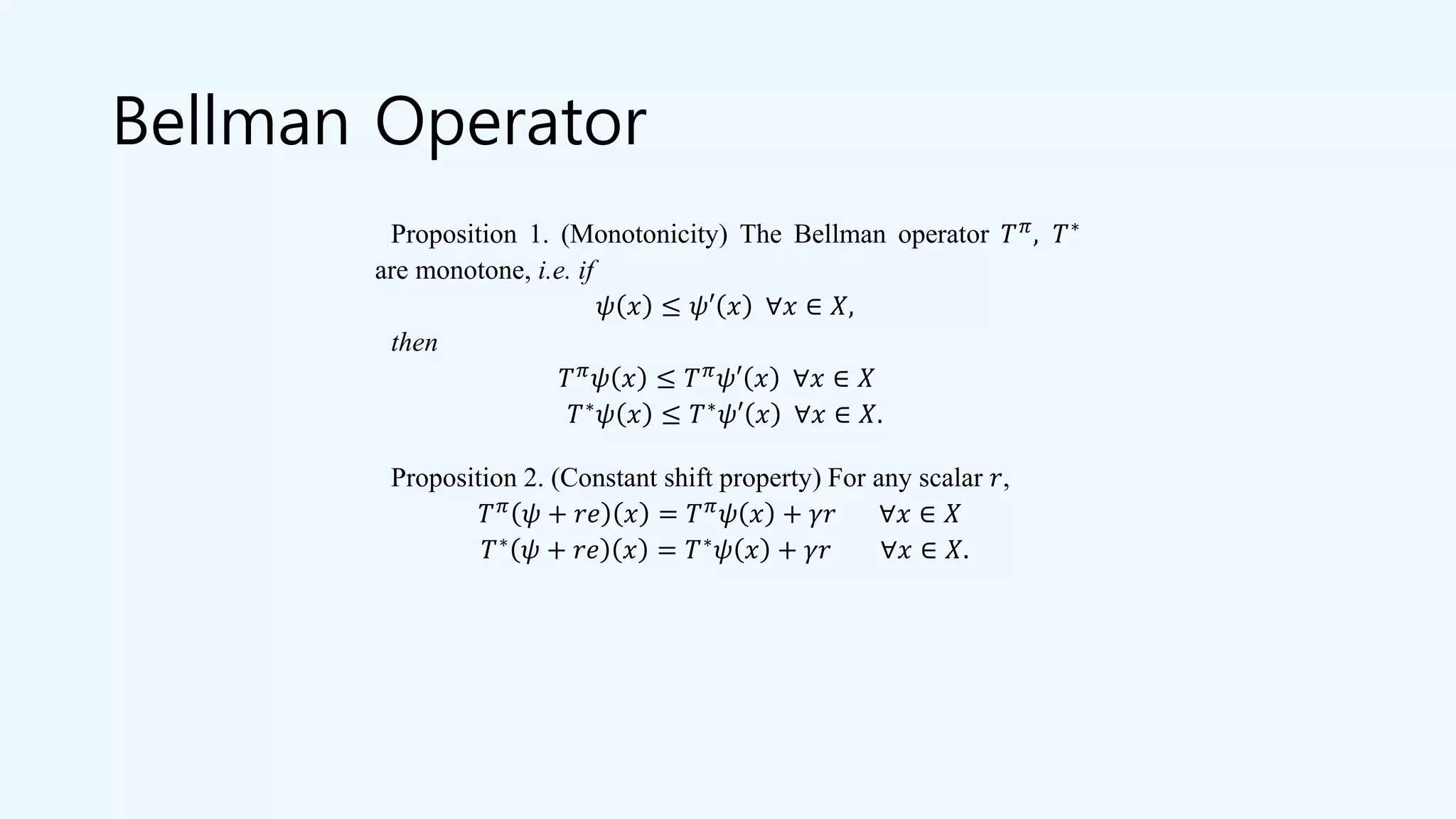
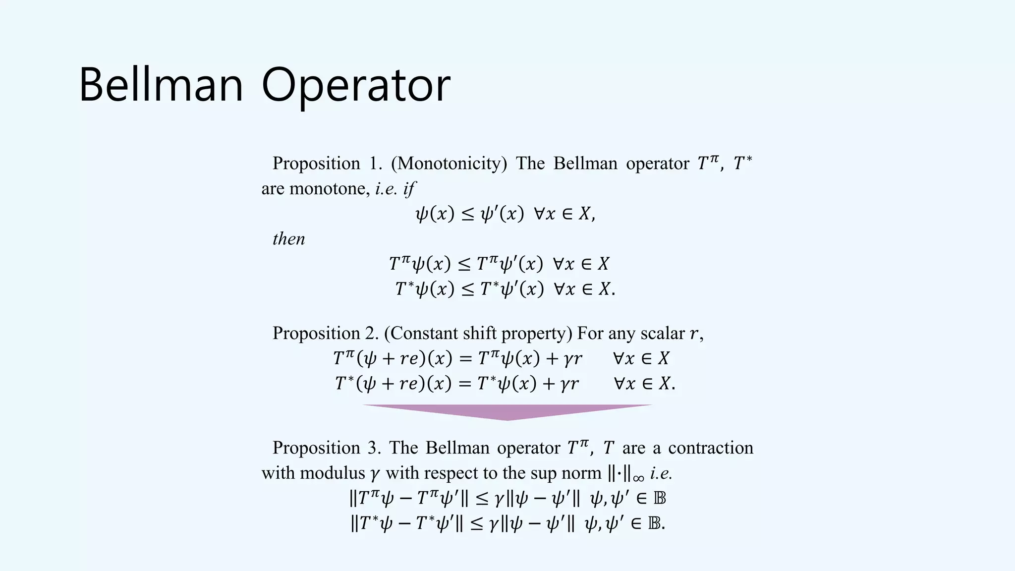
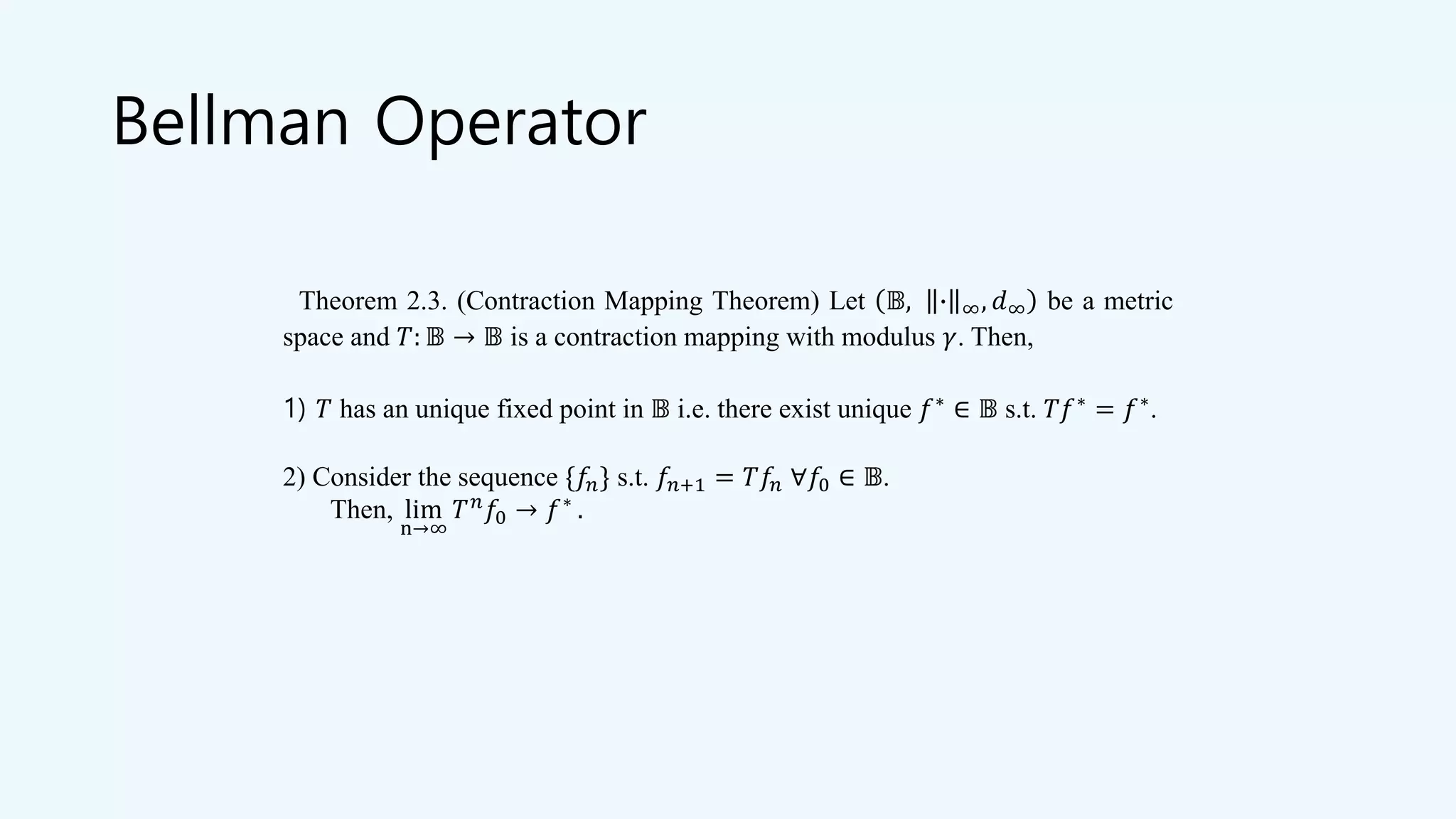
Let 𝔹, ∙ ∞, 𝑑∞ be a metric space where 𝔹 = 𝜓: Ω → ℝ continuous and bounded ,
𝜓 ∞ ≔ sup
𝑥∈𝑋
𝜓(𝑥) , and 𝑑∞ 𝜓, 𝜓′ = sup
𝑥∈𝑋
𝜓 𝑥 − 𝜓′(𝑥) .
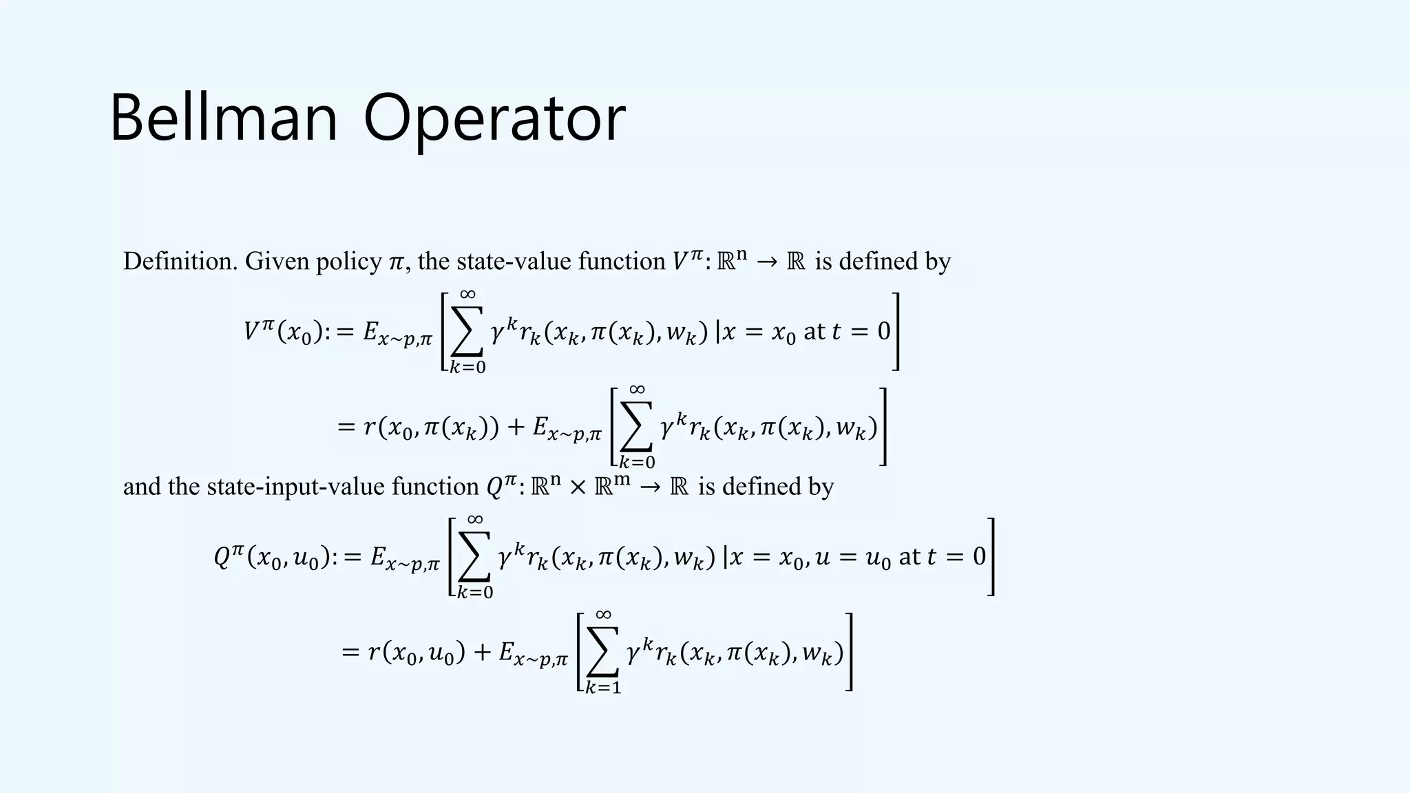
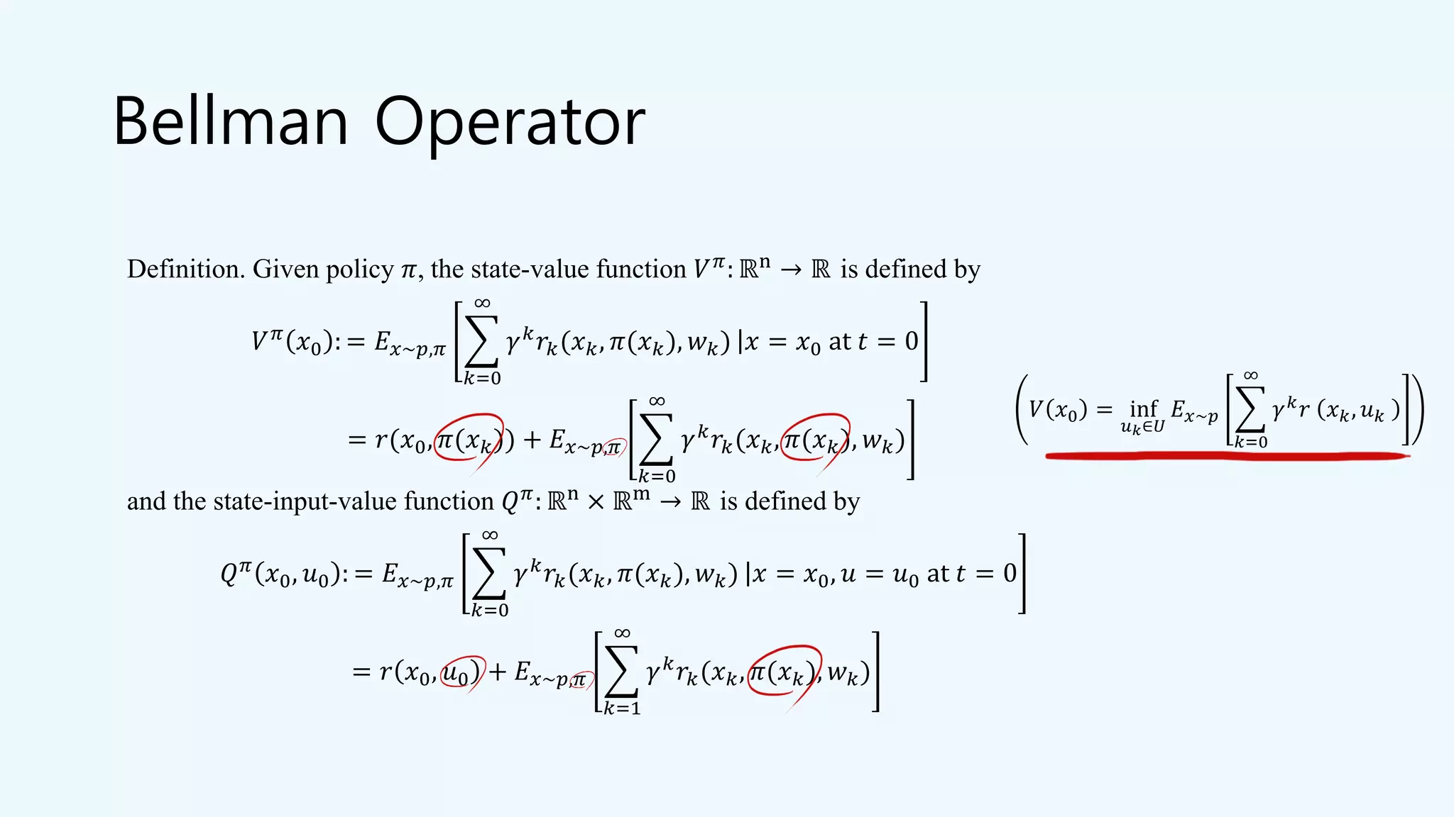
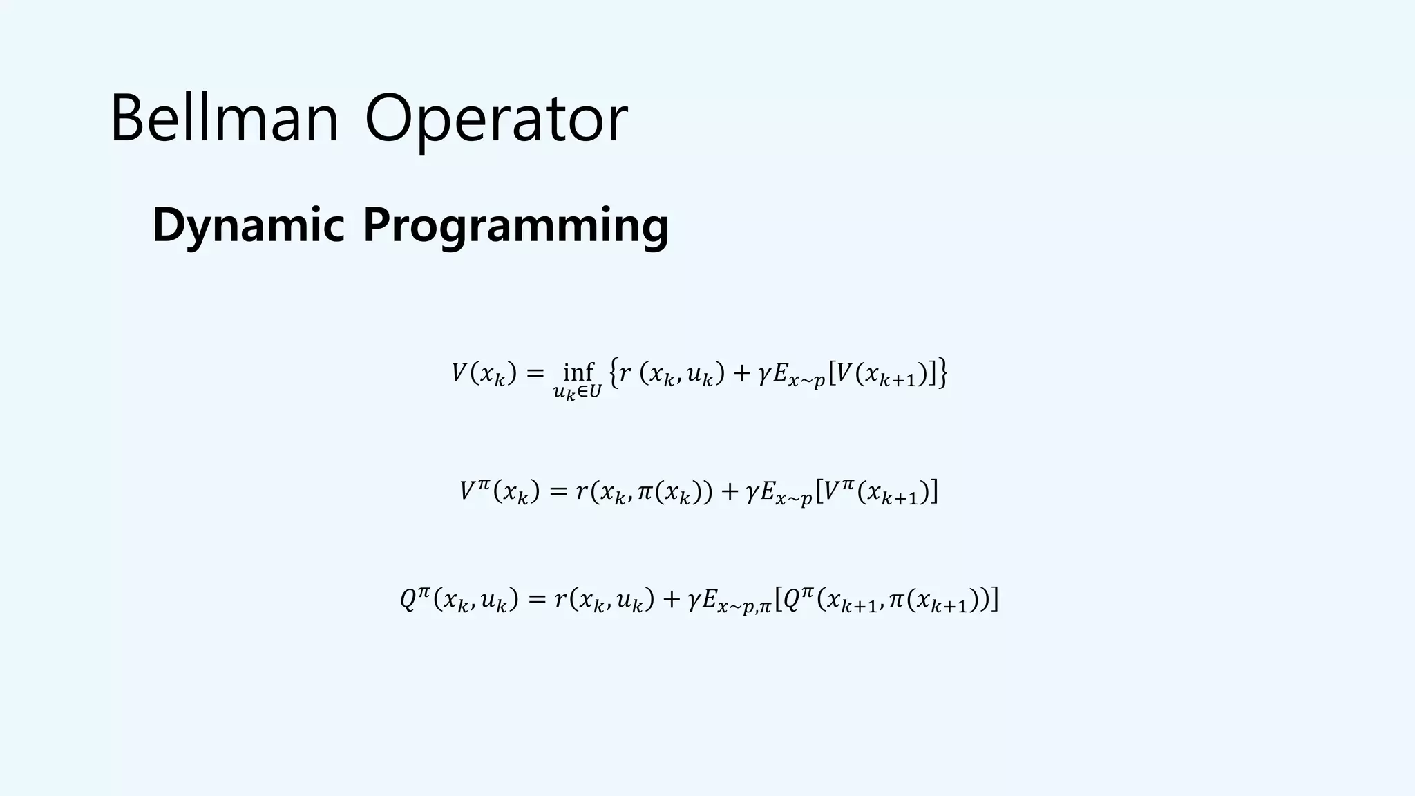
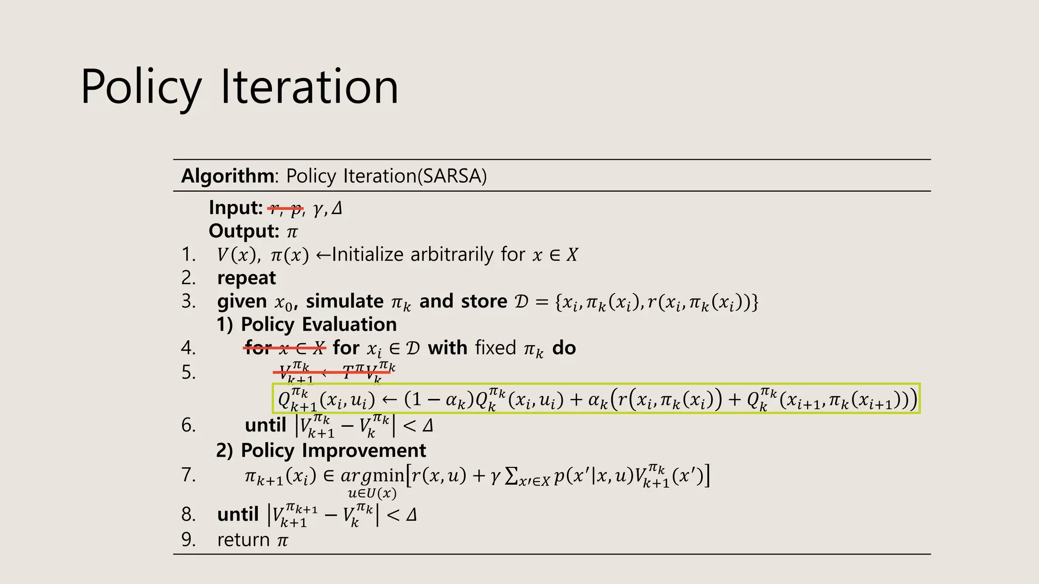
Definition. Given policy 𝜋, the Bellman operator 𝑇 𝜋: 𝔹 → 𝔹 is defined by
𝑇 𝜋 𝜓 𝑥 𝑘 = 𝑟 𝑥 𝑘, 𝜋 𝑥 𝑘 + 𝛾𝐸 𝑥~𝑝[𝜓 𝑥 𝑘+1 ]
and the Bellman optimal operator 𝑇∗: 𝔹 → 𝔹 is defined by
𝑇∗ 𝜓 𝑥 𝑘 = min
𝑢 𝑘∈𝑈(𝑥 𝑘)
𝑟 𝑥 𝑘, 𝑢 𝑘 + 𝛾𝐸 𝑥~𝑝[𝜓 𝑥 𝑘+1 ]](https://image.slidesharecdn.com/stochasticoptimalcontrolrl-200601150308/75/Stochastic-optimal-control-amp-rl-32-2048.jpg)

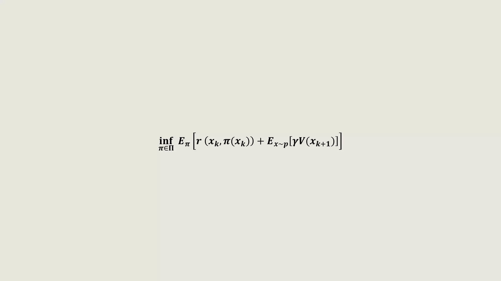
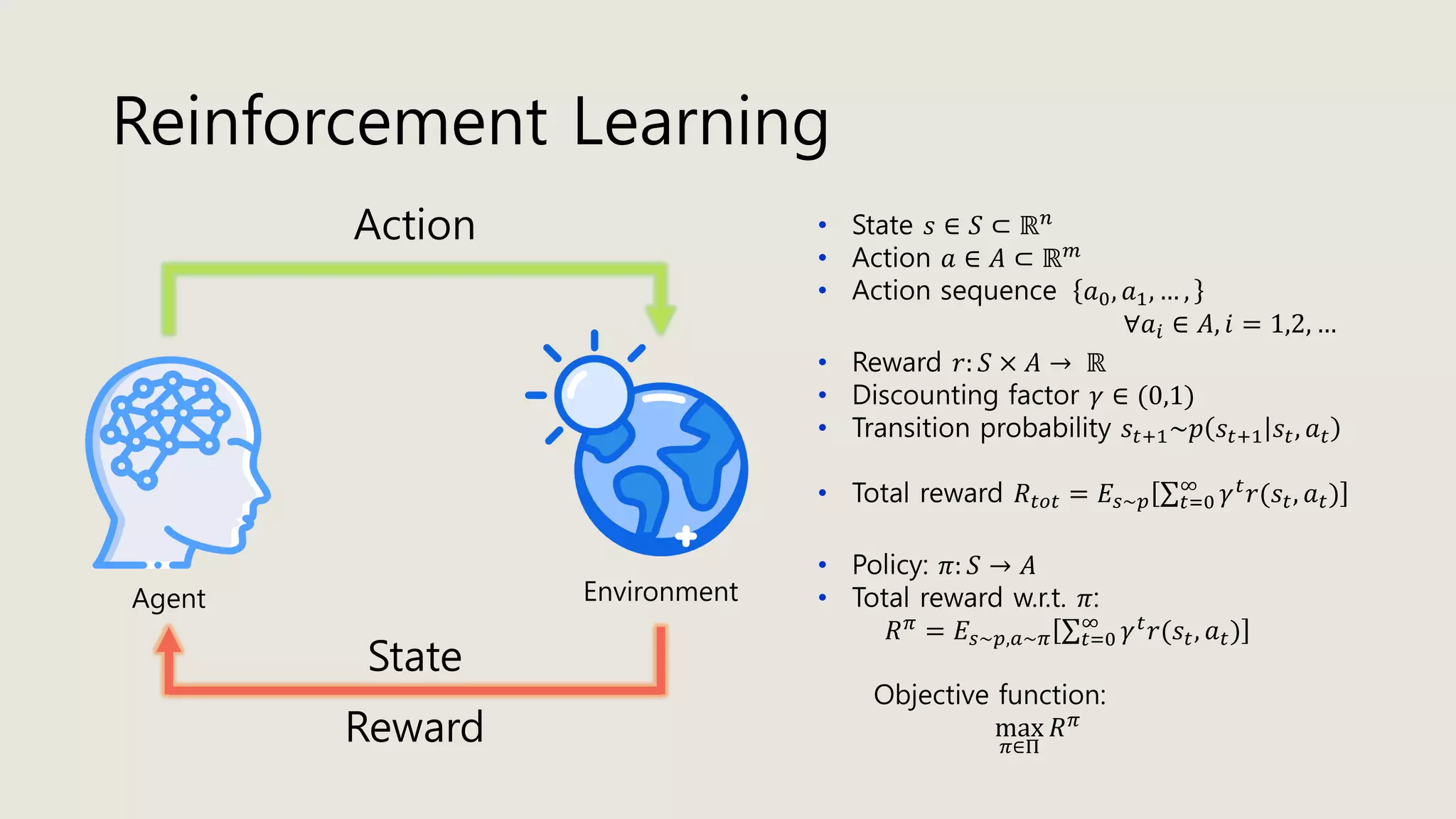
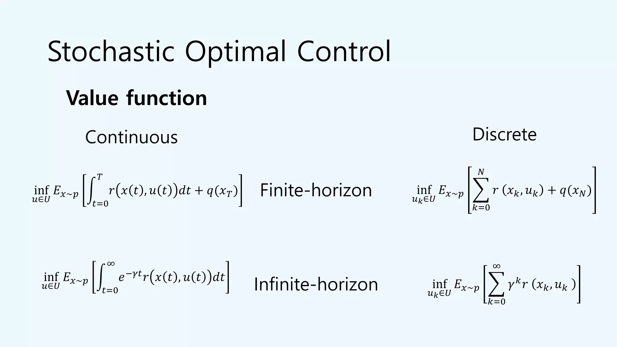
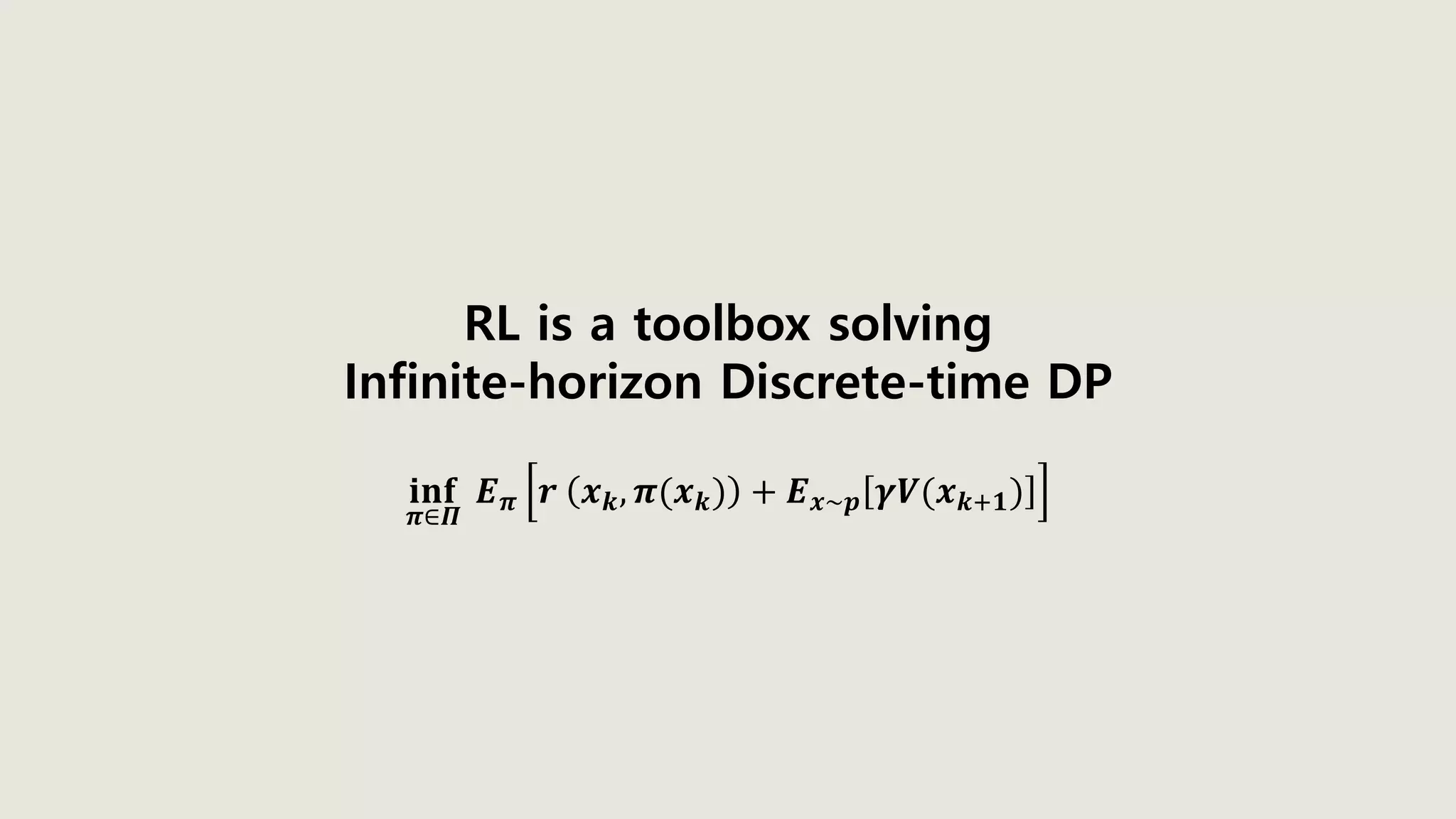
![𝐢𝐧𝐟
𝝅∈𝚷
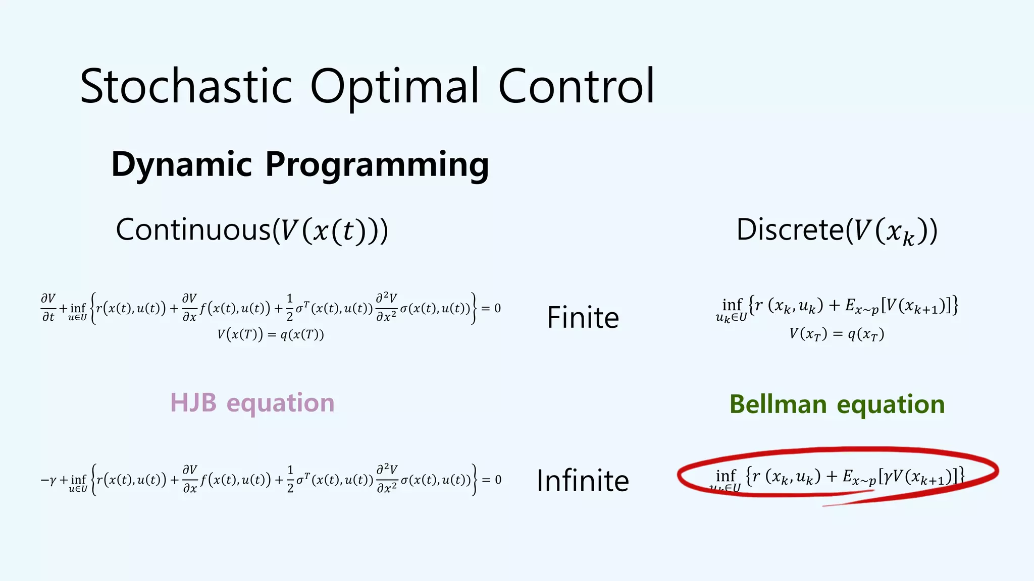
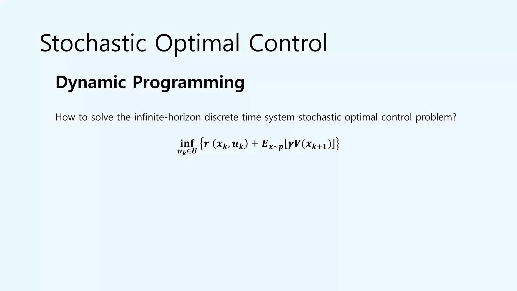
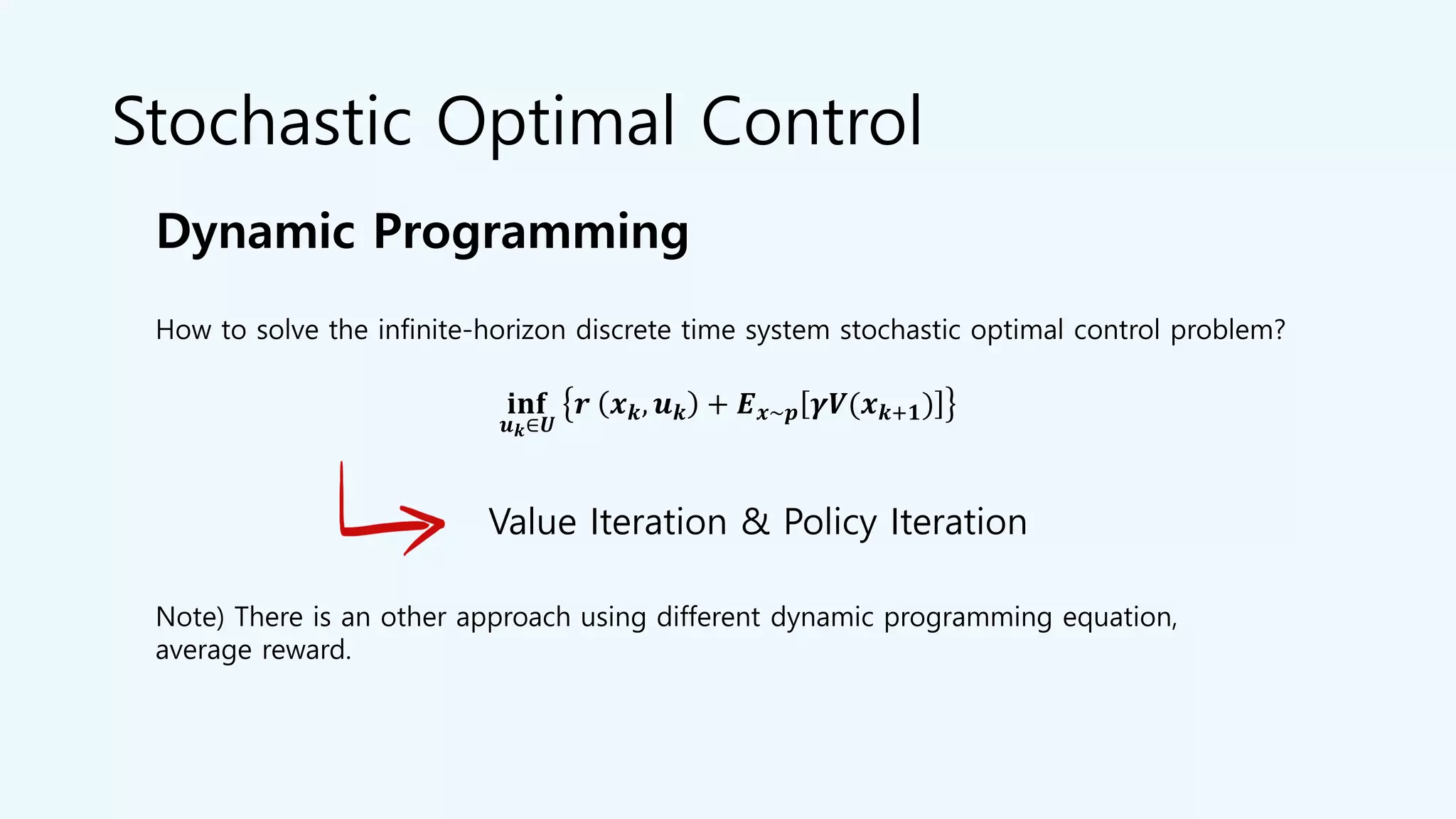
𝑬 𝝅 𝒓 𝒙 𝒌, 𝝅(𝒙 𝒌) + 𝑬 𝒙~𝒑 𝜸𝑽(𝒙 𝒌+𝟏)
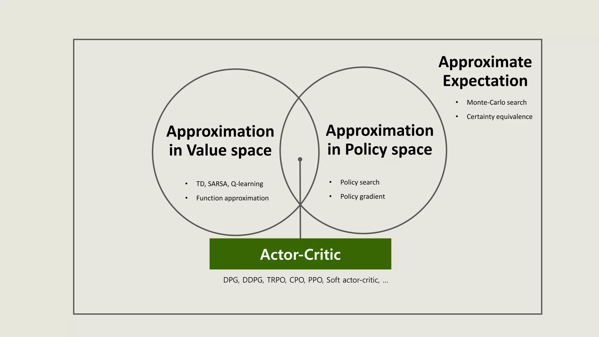
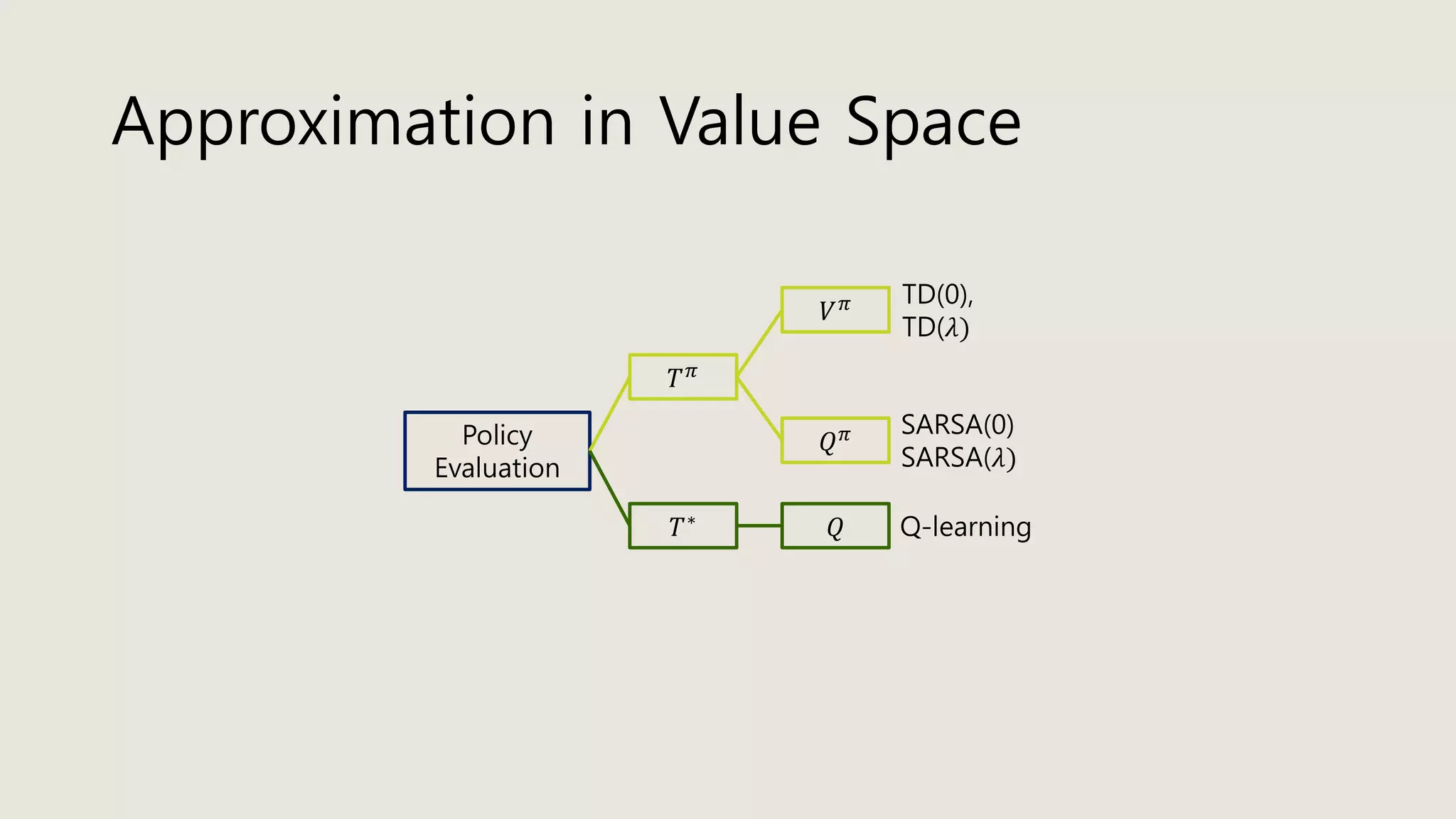
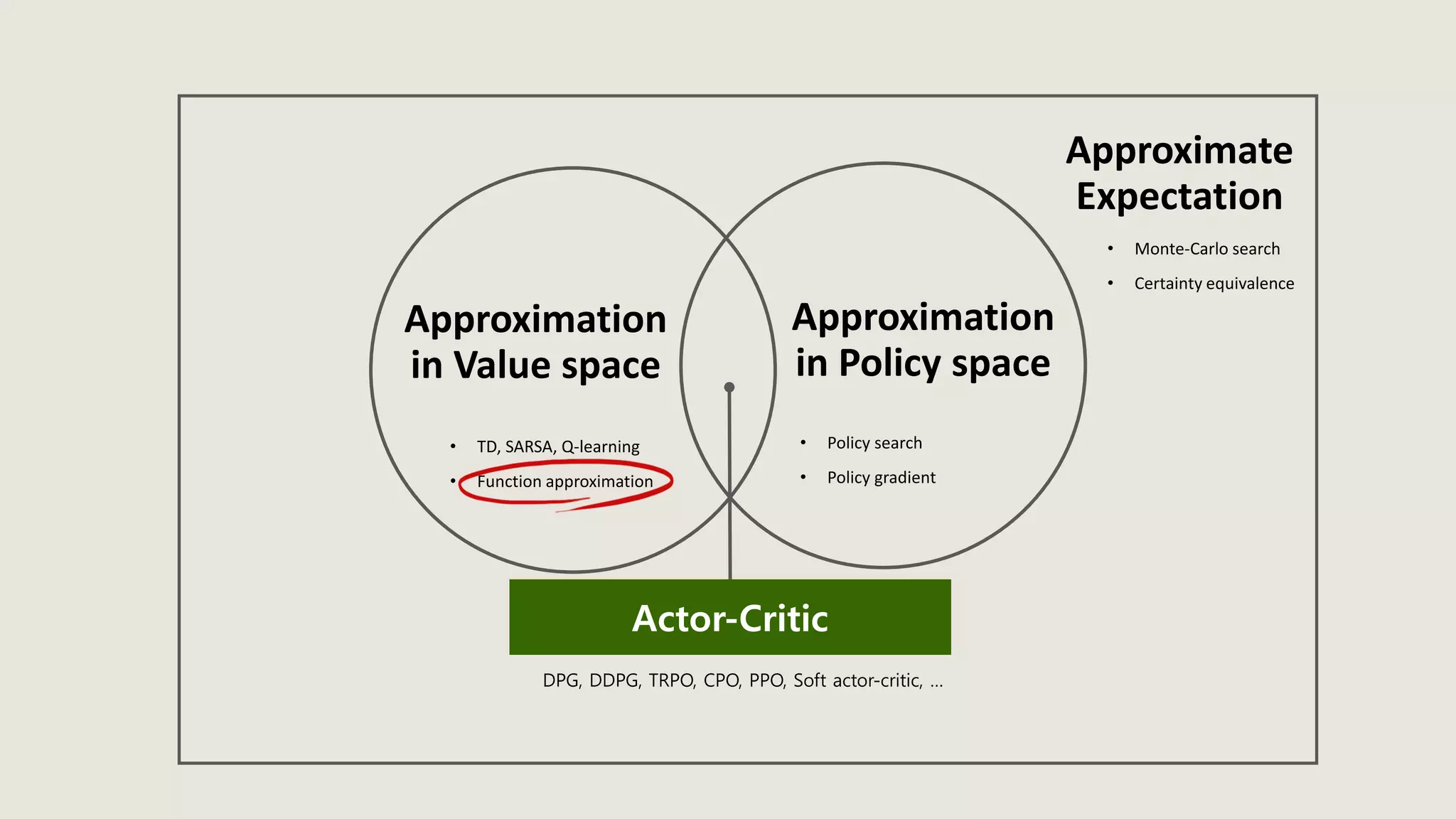
Approximation in policy space
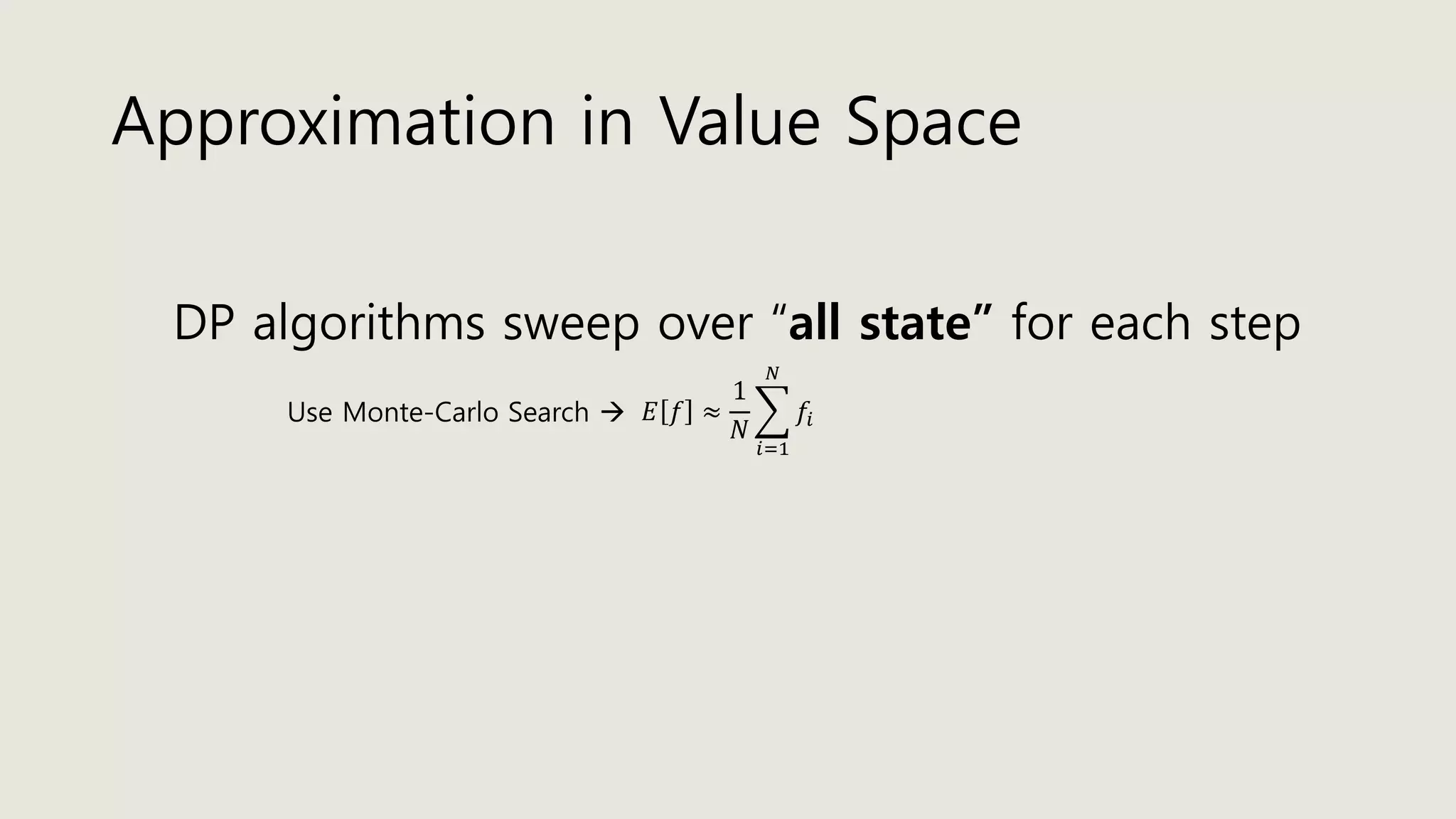
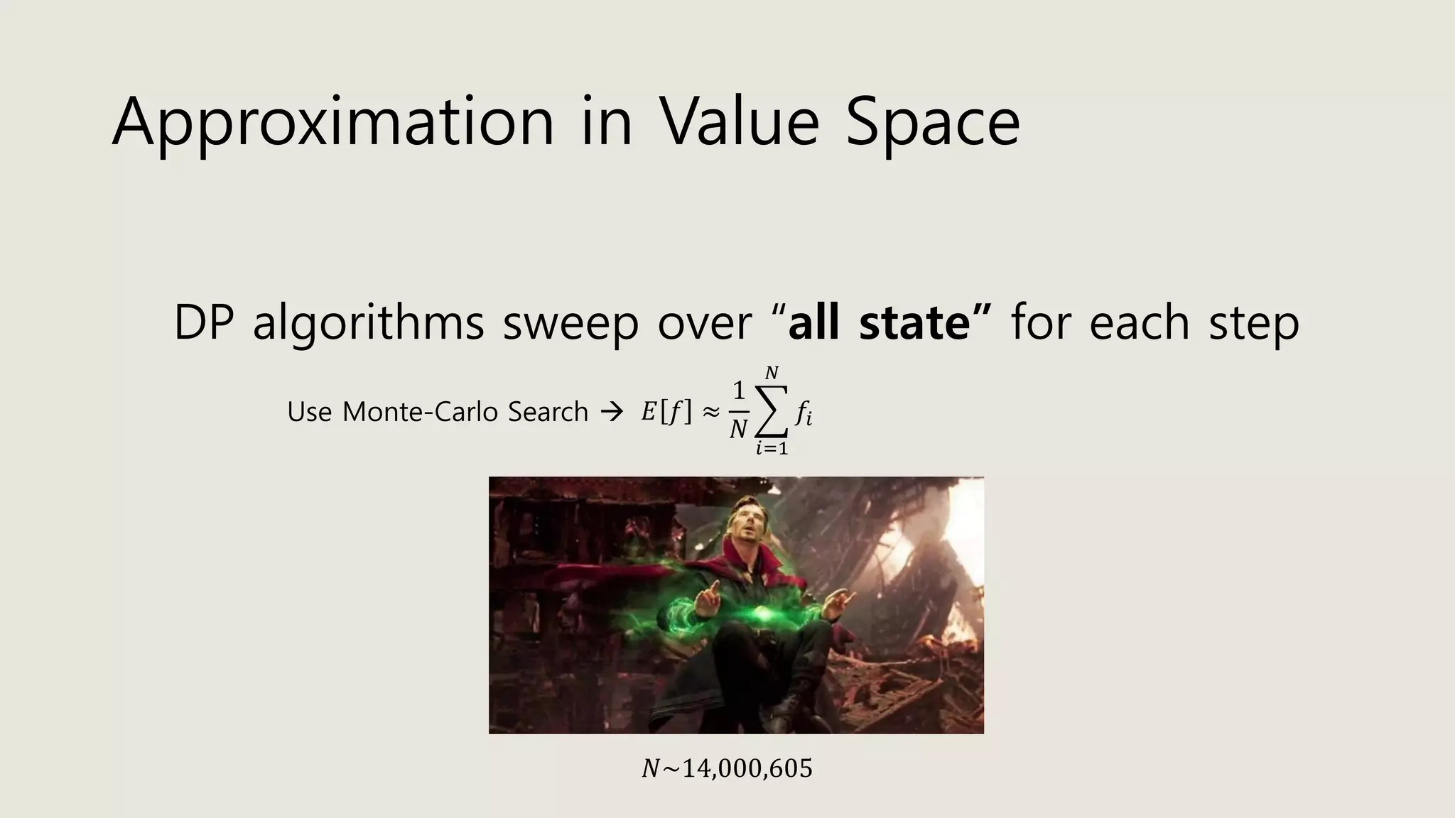
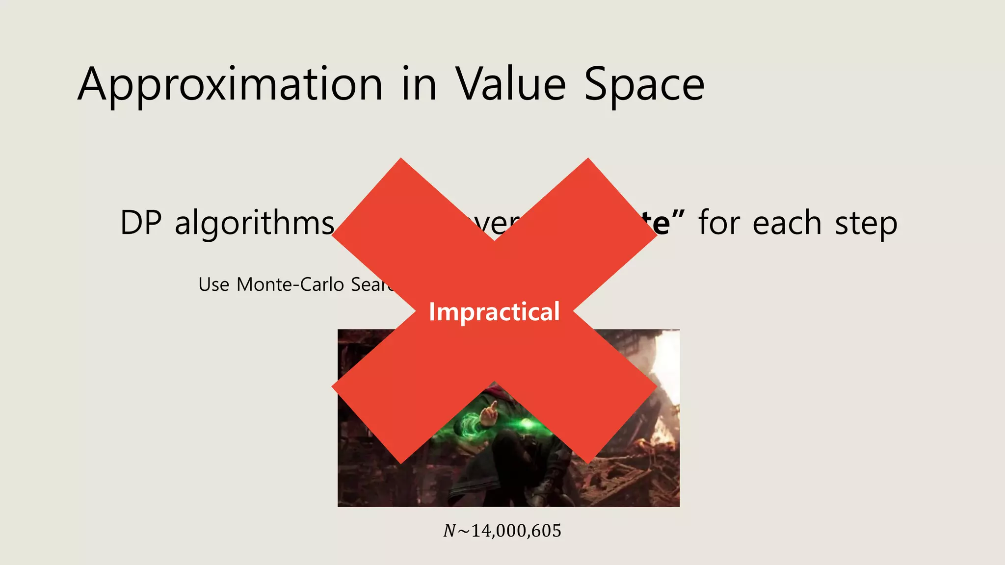
Approximation in value space
Approximate 𝐸[∙]
Parametric approximation
Problem approximation
Rollout, MPC
Monte-Carlo search
Certainty equivalence
Policy search
Policy gradient](https://image.slidesharecdn.com/stochasticoptimalcontrolrl-200601150308/75/Stochastic-optimal-control-amp-rl-44-2048.jpg)


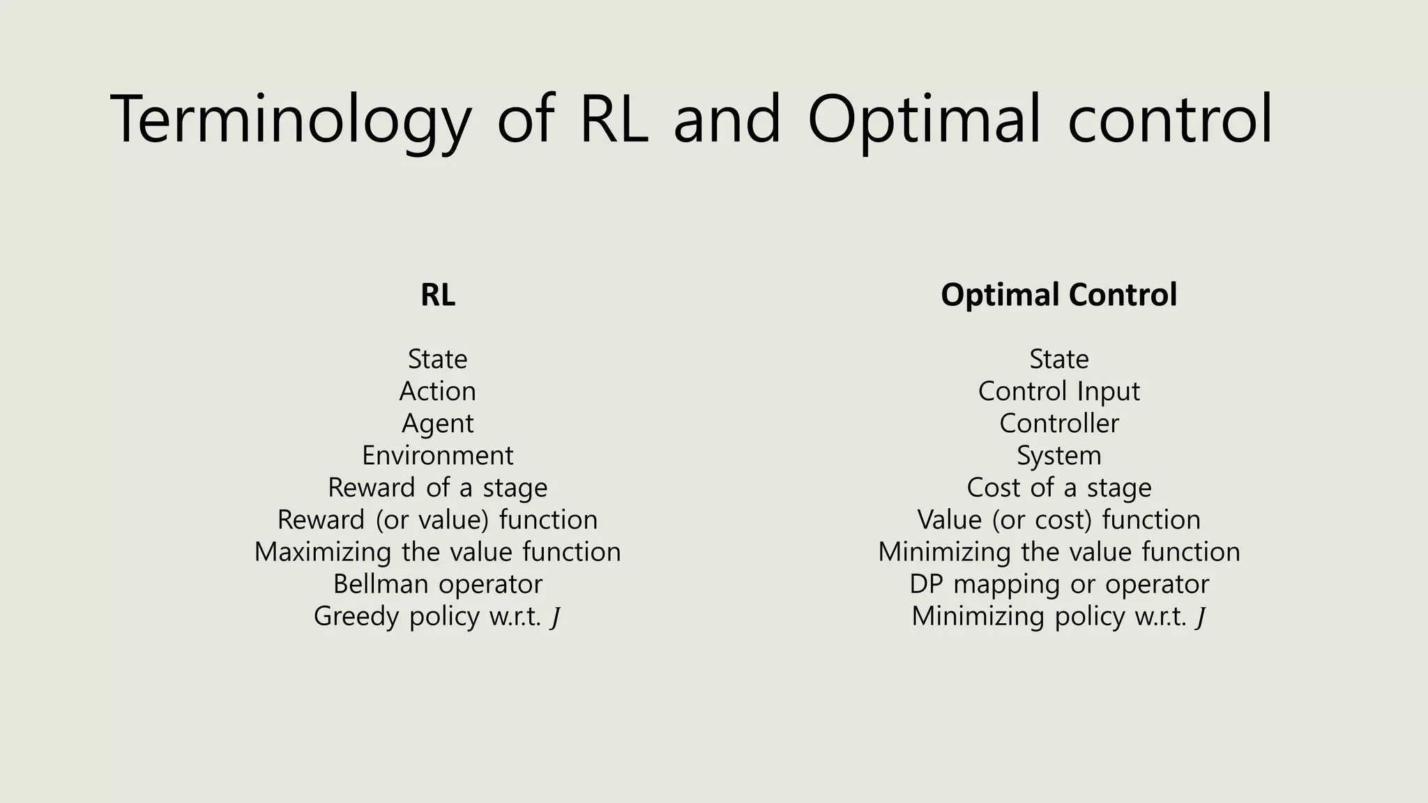
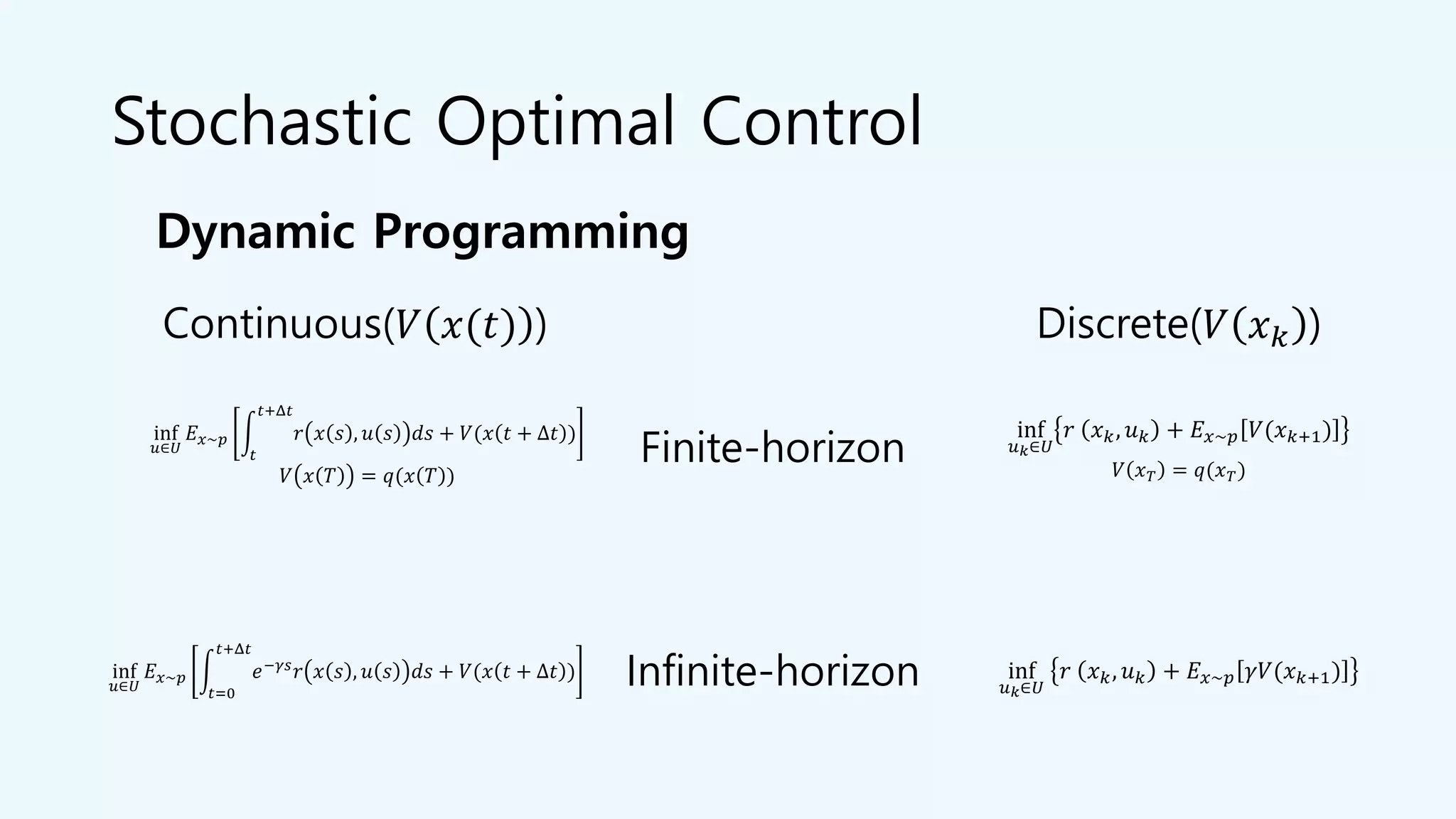
![𝐢𝐧𝐟
𝝅∈𝚷
𝑬 𝝅 𝒓 𝒙 𝒌, 𝝅(𝒙 𝒌) + 𝑬 𝒙~𝒑 𝜸𝑽(𝒙 𝒌+𝟏)
Approximation in policy space
Approximation in value space
Approximate 𝐸[∙]
Parametric approximation
Problem approximation
Rollout, MPC
Monte-Carlo search
Certainty equivalence
Policy search
Policy gradient](https://image.slidesharecdn.com/stochasticoptimalcontrolrl-200601150308/75/Stochastic-optimal-control-amp-rl-66-2048.jpg)


![Av 738- Adaptive Filtering - Wiener Filters[wk 3]](https://cdn.slidesharecdn.com/ss_thumbnails/av-738-aft-spr18-lecture03-optimumfilters-weinerwk3-180215235757-thumbnail.jpg?width=640&height=640&fit=bounds)