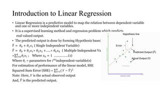
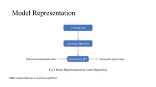
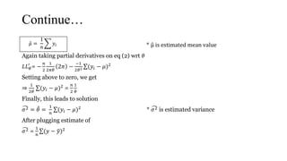
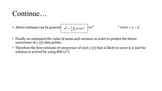
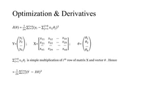
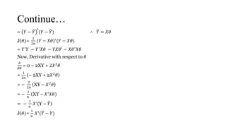
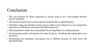
The document provides an overview of linear regression as a predictive model that establishes relationships between dependent and independent variables using cost functions and gradient descent for optimization. It explains concepts such as hypothesis representation, error calculation, maximum likelihood estimation for mean and variance, and the workings of gradient descent, including steps to adjust parameter values. The conclusion emphasizes that linear regression's cost function is convex, ensuring convergence to a global optimum without local optima.

1. Linear Regression, Costs & Gradient Descent
Pallavi Mishra
&
Revanth Kumar

2. Introduction to Linear Regression
• Linear Regression is a predictive model to map the relation between dependent variable
and one or more independent variables.
• It is a supervised learning method and regression problem which predicts
real valued output.
• The predicted output is done by forming Hypothesis based on learning algo.
𝑌 = 𝜃0 + 𝜃1 𝑥1 ( Single Independent Variable)
𝑌 = 𝜃0 + 𝜃1 𝑥1+ 𝜃2 𝑥2 +…..+ 𝜃 𝑘 𝑥 𝑘 ( Multiple Independent Variables)
= 𝑖=0
𝑘
𝜃𝑖 𝑥𝑖 ; Where 𝑥0 = 1 …………….(1)
Where 𝜃𝑖 = parameters for 𝑖 𝑡ℎindependent variable(s)
For estimation of performance of the linear model, SSE
Squared Sum Error (SSE) = 𝑖=1
𝑘
( 𝑌 − 𝑌)2
Note: Here, 𝑌 is the actual observed output
And, 𝑌 is the predicted output.
Hypothesis line
Actual Output (Y)
Predicted Output ( 𝑌)
Error

3. Model Representation
Training Set
Learning Algorithm
Hypothesis ( 𝑌)Unknown Independent Value Estimated Output Value
Fig.1 Model Representation of Linear Regression
Hint: Gradient descent as learning algorithm

4. How to Represent Hypothesis?
• We know, hypothesis is represented by 𝑌, which can be formulated
depending upon single variable linear regression (Univariate Linear
Regression) or Multi-variate linear regression.
• 𝑌 = 𝜃0 + 𝜃1 𝑥1
• Here, 𝜃0 = intercept and 𝜃1 = slope=
Δ𝑦
Δ𝑥
and 𝑥1 = independent variable
• Question arises: How do we choose 𝜃𝑖′ 𝑠 values for best fitting hypothesis?
• Idea : Choose 𝜃0 , 𝜃1 so that 𝑌 is close to 𝑌 for our training examples (x, y)
• Objective: min J(𝜃0 , 𝜃1 ),
• Note: J(𝜃0 , 𝜃1 ) = Cost Function.
• Formulation of J(𝜃0 , 𝜃1 ) =
1
2𝑚 𝑖=1
𝑚
( 𝑌(𝑖)−𝑌(𝑖))
2
Note: m = No. of instances of dataset

5. Objective function for linear regression
• The most important objective of linear regression model is to minimize cost function by
choosing a optimal value for 𝜃0 , 𝜃1.
• For optimization technique, Gradient Descent is mostly used in case of predictive models.
• By taking 𝜃0 = 0 and 𝜃1 = some random values ( in case of univariate linear regression),
the graph (𝜃1 vs J(𝜃1 )) gets represented in the form of bow shaped.
Advantage of Gradient descent in linear regression model
• No scope to stuck in local optima, since there is only
One global optima position where slope(𝜃1) = 0
(convex graph)
𝜃1
𝐽(𝜃1)

6. Normal Distribution N(𝜇, 𝜎2
)
Estimation of mean (𝝁) and variance (𝝈 𝟐):
• Let size of data set = n, denoted by 𝑦1, 𝑦2…… 𝑦𝑛
• Assuming 𝑦1, 𝑦2…… 𝑦𝑛 are independent random variables or Independent Identically
Distributed (iid), they are normally distributed random variables.
• Assuming no independent variables (x), in order to estimate the future value of y we need to find
to find unknown parameters (𝜇 & 𝜎2).
Concept of Maximum Likelihood Estimation:
• Using Maximum Likelihood Estimation (MLE) concept, we are trying to find the optimal value for
value for the mean (𝜇) and standard deviation (σ) for distribution given a bunch of observed
observed measurements.
• The goal of MLE is to find optimal way to fit a distribution to the data so, as to work easily with
with data

7. Continue…
Estimation of 𝝁 & 𝝈 𝟐
:
• Density of normal random variable = f(y) =
1
2𝜋𝜎
𝑒
−1
2𝜎2(𝑦−𝜇)2
L (𝜇, 𝜎2
) is a joint density
Now,
let, L (𝜇, 𝜎2
) = f (𝑦1, 𝑦2…… 𝑦 𝑛) = 𝑖=1
𝑛 1
2𝜋𝜎
𝑒
−1
2𝜎2(𝑦−𝜇)2
let, assume 𝜎2 = 𝜃
let, L (𝜇, 𝜃) =
1
( 2𝜋𝜃)
𝑛 𝑒
−1
2𝜃
(𝑦−𝜇)2
taking log on both sides
LL (𝜇, 𝜃) = log (2𝜋𝜃)−
𝑛
2 + log (𝑒
−1
2𝜎2(𝑦−𝜇)2
) ∗LL (𝜇, 𝜃) is denoted as log of joint density
=−
𝑛
2
log 2𝜋𝜃 −
1
2𝜃
(𝑦 − 𝜇)2
(2) ∗ 𝑙𝑜𝑔𝑒 𝑥
= 𝑥

8. Continue…
• Our objective is to estimate the next occurring of data point y in the distribution of data.
Using MLE we can find the optimal value for (μ, σ2). For a given trainings set we need to
find max LL (μ, θ) .
• Let us assume 𝜃 = 𝜎2
for simplicity
• Now, we use partial derivatives to find the optimal values of (μ, σ2) and equating to zero
𝐿𝐿′ = 0
LL (𝜇, 𝜃) = −
𝑛
2
log 2𝜋𝜃 −
1
2𝜃
(𝑦 − 𝜇)2
• Taking partial derivative wrt 𝜇 in eq (2), we get
𝐿𝐿 𝜇
′
= 0 −
2
2𝜃
(𝑦𝑖 − 𝜇) (-1)
=> (𝑦𝑖 − 𝜇) = 0 * 𝐿𝐿 𝜇
′
is partial derivative of LL wrt 𝜇
=> 𝑦𝑖 = 𝑛 𝜇

9. Continue…
𝜇 =
1
𝑛
𝑦𝑖 * μ is estimated mean value
Again taking partial derivatives on eq (2) wrt 𝜃
𝐿𝐿 𝜃
′
= −
𝑛
2
1
2𝜋𝜃
2𝜋 −
−1
2𝜃2 (𝑦𝑖 − 𝜇)2
Setting above to zero, we get
⇒
1
2𝜃
(𝑦𝑖 − 𝜇)2 =
𝑛
2
1
𝜃
Finally, this leads to solution
𝜎2 = 𝜃 =
1
𝑛
(𝑦𝑖 − 𝜇)2 * 𝜎2 is estimated variance
After plugging estimate of
𝜎2 =
1
𝑛
(𝑦 − 𝑦)2
𝜇 =
1
𝑛
𝑦𝑖

10. Continue…
• Above estimate can be generalized to 𝜎2 =
1
𝑛
𝑒𝑟𝑟𝑜𝑟2 * error = y − 𝑦
• Finally we estimated the value of mean and variance in order to predict the future
occurrence of y ( 𝑦) data points.
• Therefore the best estimate of occurrence of next y ( 𝑦) that is likely to occur is 𝜇 and the
solution is arrived by using SSE ( 𝜎2)
𝜎2 =
1
𝑛
𝑒𝑟𝑟𝑜𝑟2

11. Optimization & Derivatives
J(𝜃) =
1
2𝑛 𝑖=1
𝑖=𝑛
(𝑦𝑖 − 𝑗=1
𝑗=𝑘
𝑥𝑖𝑗 𝜃𝑗)2
Y=
𝑦1
𝑦2
…
𝑦𝑛
; X=
𝑥11 𝑥12 … 𝑥1𝑘
𝑥21 𝑥22 … 𝑥2𝑘
…
𝑥 𝑛1
…
𝑥2𝑛
… …
… 𝑥 𝑛𝑘
; 𝜃=
𝜃1
𝜃2
…
𝜃 𝑘
𝑗=1
𝑗=𝑘
𝑥𝑖𝑗 𝜃𝑗 is simple multiplication of 𝑖 𝑡ℎ
row of matrix X and vector 𝜃 . Hence
=
1
2𝑛 𝑖=1
𝑖=𝑛
(𝑌 − 𝑋𝜃)2

12. Continue…
= 𝑌 − 𝑌
′
(𝑌 − 𝑌) ∴ 𝑌 = 𝑋𝜃
J(𝜃)=
1
2𝑛
𝑌 − 𝑋𝜃 ′(𝑌 − 𝑋𝜃)
= 𝑌′
𝑌 − 𝑌′
𝑋𝜃 − 𝑌𝑋𝜃′
− 𝑋𝜃′
𝑋𝜃
Now, Derivative with respect to 𝜃
𝜕
𝜕𝜃
= 0 – 2XY + 2𝑋2 𝜃
=
1
2𝑛
(– 2XY + 2𝑋2 𝜃)
= −
2
2𝑛
(XY – 𝑋2 𝜃)
= −
1
𝑛
(XY – 𝑋′ 𝑋𝜃)
= −
1
𝑛
𝑋′
(Y – 𝑌)
J(𝜃)=
1
𝑛
𝑋′( 𝑌 − 𝑌)

13. How to start with Gradient Descent
• The basic assumption is to start at any random position 𝑥0 and take derivative value.
• 1 𝑠𝑡 case: if derivative value > 0 , increasing
• Action : then change the 𝜃1 values using the gradient descent formula.
• 𝜃1 = 𝜃1 - 𝛼
𝑑 𝐽(𝜃1)
𝑑𝜃1
• here, 𝛼 = learning rate / parameter

14. Gradient Descent algorithm
• Repeat until convergence { 𝜃1: = 𝜃1 - 𝛼
𝑑 𝐽(𝜃1)
𝑑𝜃1
here, assuming 𝜃0 = 0 for univariate linear
regression }
For multi variate linear regression:
• Repeat until convergence { 𝜃𝑗 := 𝜃𝑗 - 𝛼
𝑑 𝐽(𝜃0, 𝜃1)
𝑑𝜃 𝑗
}
Simultaneous update of 𝜃0, 𝜃1
Temp 0 := 𝜃 𝑜: = 𝜃0 - 𝛼
𝑑 𝐽(𝜃0, 𝜃1)
𝑑𝜃0
Temp 1 := 𝜃1: = 𝜃1 - 𝛼
𝑑 𝐽(𝜃0, 𝜃1)
𝑑𝜃1
𝜃 𝑜: = Temp 0
𝜃1: = Temp 1

15. Effects associated with varying values of
learning rate (𝛼)
𝛼

16. Continue:
• In the first case, we may find difficulty to reach at global optima since large value of 𝛼 may
overshoot the optimal position due to aggressive updating of 𝜃 values.
• Therefore, as we approach optima position, gradient descent will take automatically
smaller steps.

17. Conclusion
• The cost function for linear regression is always gong to be a bow-shaped function
(convex function)
• This function doesn’t have an local optima except for the one global optima.
• Therefore, using cost function of type 𝐽(𝜃0, 𝜃1) which we get whenever we are using linear
regression, it will always converge to the global optimum.
• Most important is make sure our gradient descent algorithms is working properly .
• On increasing number of iterations, the value of 𝐽(𝜃0, 𝜃1) should get decreasing after every
iterations.
• Determining the automatic convergence test is difficult because we don't know the
threshold value.