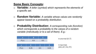
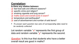
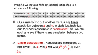
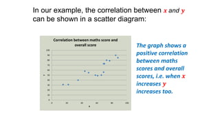
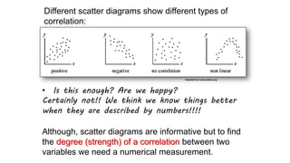
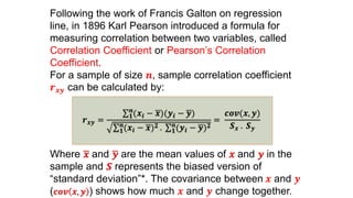
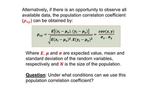
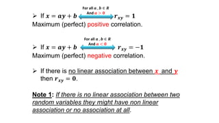
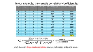
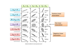
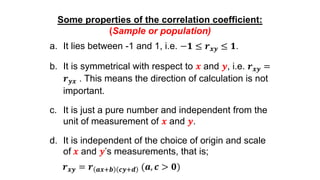
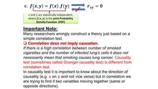
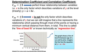
This document provides an introduction to correlation and regression analysis. It defines key concepts like variables, random variables, and probability distributions. It discusses how correlation measures the strength and direction of a linear relationship between two variables. Correlation coefficients range from -1 to 1, with values closer to these extremes indicating stronger correlation. The document also introduces determination coefficients, which measure the proportion of variance in one variable explained by the other. Regression analysis builds on correlation to study and predict the average value of one variable based on the values of other explanatory variables.

1. Introduction to Correlation &
Regression Analysis
Farzad Javidanrad
November 2013

2. Some Basic Concepts:
o Variable: A letter (symbol) which represents the elements of
a specific set.
o Random Variable: A variable whose values are randomly
appear based on a probability distribution.
o Probability Distribution: A corresponding rule (function)
which corresponds a probability to the values of a random
variable (individually or to a set of them). E.g.:
𝒙 0 1
𝑃(𝑥) 0.5 0.5
In one trial 𝐻, 𝑇
In two trials
𝐻𝐻, 𝐻𝑇, 𝑇𝐻, 𝑇𝑇

3. Correlation:
Is there any relation between:
 fast food sale and different seasons?
 specific crime and religion?
 smoking cigarette and lung cancer?
 maths score and overall score in exam?
 temperature and earthquake?
 cost of advertisement and number of sold items?
 To answer each question two sets of corresponding data need to
be randomly collected.
Let random variable "𝒙" represents the first group of
data and random variable "𝒚" represents the second.
Question: Is this true that students who have a better
overall result are good in maths?

4. Our aim is to find out whether there is any linear
association between 𝒙 and 𝒚. In statistics, technical
term for linear association is “correlation”. So, we are
looking to see if there is any correlation between two
scores.
 “Linear association” : variables are in relations at
their levels, i.e. 𝒙 with 𝒚 not with 𝒚 𝟐
, 𝒚 𝟑
,
𝟏
𝒚
or even
∆𝒚.
Imagine we have a random sample of scores in a
school as following:

5. In our example, the correlation between 𝒙 and 𝒚
can be shown in a scatter diagram:
0
10
20
30
40
50
60
70
80
90
100
0 20 40 60 80 100
Y
X
Correlation between maths score and
overall score The graph shows a
positive correlation
between maths
scores and overall
scores, i.e. when 𝒙
increases 𝒚
increases too.

6. Different scatter diagrams show different types of
correlation:
• Is this enough? Are we happy?
Certainly not!! We think we know things better
when they are described by numbers!!!!
Although, scatter diagrams are informative but to find
the degree (strength) of a correlation between two
variables we need a numerical measurement.
Adopted from www.pdesas.org

7. Following the work of Francis Galton on regression
line, in 1896 Karl Pearson introduced a formula for
measuring correlation between two variables, called
Correlation Coefficient or Pearson’s Correlation
Coefficient.
For a sample of size 𝒏, sample correlation coefficient
𝒓 𝒙𝒚 can be calculated by:
𝒓 𝒙𝒚 =
𝟏
𝒏
(𝒙𝒊 − 𝒙)(𝒚𝒊 − 𝒚)
𝟏
𝒏
(𝒙𝒊 − 𝒙) 𝟐 . 𝟏
𝒏
(𝒚𝒊 − 𝒚) 𝟐
=
𝒄𝒐𝒗(𝒙, 𝒚)
𝑺 𝒙 . 𝑺 𝒚
Where 𝒙 and 𝒚 are the mean values of 𝒙 and 𝒚 in the
sample and 𝑺 represents the biased version of
“standard deviation”*. The covariance between 𝒙 and 𝒚
( 𝒄𝒐𝒗 𝒙, 𝒚 ) shows how much 𝒙 and 𝒚 change together.

8. Alternatively, if there is an opportunity to observe all
available data, the population correlation coefficient
(𝝆 𝒙𝒚) can be obtained by:
𝝆 𝒙𝒚 =
𝑬 𝒙𝒊 − 𝝁 𝒙 . (𝒚𝒊 − 𝝁 𝒚)
𝑬 𝒙𝒊 − 𝝁 𝒙
𝟐. 𝑬(𝒚𝒊 − 𝝁 𝒚) 𝟐
=
𝒄𝒐𝒗(𝒙, 𝒚)
𝝈 𝒙 . 𝝈 𝒚
Where 𝑬, 𝝁 and 𝝈 are expected value, mean and
standard deviation of the random variables,
respectively and 𝑵 is the size of the population.
Question: Under what conditions can we use this
population correlation coefficient?

9.  If 𝒙 = 𝒂𝒚 + 𝒃 𝒓 𝒙𝒚 = 𝟏
Maximum (perfect) positive correlation.
 If 𝒙 = 𝒂𝒚 + 𝒃 𝒓 𝒙𝒚 = −𝟏
Maximum (perfect) negative correlation.
 If there is no linear association between 𝒙 and 𝒚
then 𝒓 𝒙𝒚 = 𝟎.
Note 1: If there is no linear association between two
random variables they might have non linear
association or no association at all.
For all 𝒂 , 𝒃 ∈ 𝑹
And 𝒂 > 𝟎
For all 𝒂 , 𝒃 ∈ 𝑹
And 𝒂 < 𝟎

10. In our example, the sample correlation coefficient is:
𝒙𝒊 𝒚𝒊 𝒙𝒊 − 𝒙 𝒚𝒊 − 𝒚 𝒙𝒊 − 𝒙 . (𝒚𝒊 − 𝒚) (𝑥𝑖− 𝑥 )2
(𝑦𝑖− 𝑦 )2
70 73 12 13.9 166.8 144 193.21
85 90 27 30.9 834.3 729 954.81
22 31 -36 -28.1 1011.6 1296 789.61
66 50 8 -9.1 -72.8 64 82.81
15 31 -43 -28.1 1208.3 1849 789.61
58 50 0 -9.1 0 0 82.81
69 56 11 -3.1 -34.1 121 9.61
49 55 -9 -4.1 36.9 81 16.81
73 80 15 20.9 313.5 225 436.81
61 49 3 -10.1 -30.3 9 102.01
77 79 19 19.9 378.1 361 396.01
44 58 -14 -1.1 15.4 196 1.21
35 40 -23 -19.1 439.3 529 364.81
88 85 30 25.9 777 900 670.81
69 73 11 13.9 152.9 121 193.21
5196.9 6625 5084.15
𝒓 𝒙𝒚 =
𝟏
𝒏
(𝒙𝒊 − 𝒙)(𝒚𝒊 − 𝒚)
𝟏
𝒏
(𝒙𝒊 − 𝒙) 𝟐 . 𝟏
𝒏
(𝒚𝒊 − 𝒚) 𝟐
= 𝟓𝟏𝟗𝟔.𝟗
𝟔𝟔𝟐𝟓×𝟓𝟎𝟖𝟒.𝟏𝟓
=𝟎.𝟖𝟗𝟓
which shows an strong positive correlation between maths score and overall score.

11. Positive Linear
Association
No Linear
Association
Negative Linear
Association
𝑺 𝒙 > 𝑺 𝒚 𝑺 𝒙 = 𝑺 𝒚 𝑺 𝒙 < 𝑺 𝒚
𝒓 𝒙𝒚 = 𝟏
Adapted and modified from www.tice.agrocampus-ouest.fr
𝒓 𝒙𝒚 ≈ 𝟏
𝟎 < 𝒓 𝒙𝒚 < 𝟏
𝒓 𝒙𝒚 = 𝟎
−𝟏 < 𝒓 𝒙𝒚< 𝟎
𝒓 𝒙𝒚 ≈ −𝟏
𝒓 𝒙𝒚 = −𝟏
Perfect
Weak
No
Correlation
Weak
Strong
Perfect
Strong

12. Some properties of the correlation coefficient:
(Sample or population)
a. It lies between -1 and 1, i.e. −𝟏 ≤ 𝒓 𝒙𝒚 ≤ 𝟏.
b. It is symmetrical with respect to 𝒙 and 𝒚, i.e. 𝒓 𝒙𝒚 =
𝒓 𝒚𝒙 . This means the direction of calculation is not
important.
c. It is just a pure number and independent from the
unit of measurement of 𝒙 and 𝒚.
d. It is independent of the choice of origin and scale
of 𝒙 and 𝒚’s measurements, that is;
𝒓 𝒙𝒚 = 𝒓 𝒂𝒙+𝒃 𝒄𝒚+𝒅 (𝒂, 𝒄 > 𝟎)

13. e. 𝒇 𝒙, 𝒚 = 𝒇 𝒙 . 𝒇(𝒚) 𝒓 𝒙𝒚 = 𝟎
Important Note:
Many researchers wrongly construct a theory just based on a
simple correlation test.
 Correlation does not imply causation.
If there is a high correlation between number of smoked
cigarettes and the number of infected lung’s cells it does not
necessarily mean that smoking causes lung cancer. Causality
test (sometimes called Granger causality test) is different from
correlation test.
In causality test it is important to know about the direction of
causality (e.g. 𝒙 on 𝒚 and not vice versa) but in correlation we
are trying to find if two variables moving together (same or
opposite directions).
𝒙 and 𝒚 are statistically independent,
where 𝒇(𝒙, 𝒚) is the joint Probability
Density Function (PDF)

14. Determination Coefficient and Correlation Coefficient:
𝒓 𝒙𝒚 = ±𝟏 perfect linear relationship between variables:
i.e. 𝒙 is the only factor which describes variations of 𝒚 at the level
(linearly); 𝒚 = 𝒂 + 𝒃𝒙 .
𝒓 𝒙𝒚 ≈ ±𝟏 𝒙 is not the only factor which describes
variations of 𝒚 but we can still imagine that a line represents this
relationship which passing through most of the points or having a
minimum vertical distance from them, in total. This line is called
the “line of best fit” or known technically as “regression line”.
Adopted from www.ncetm.org.uk/public/files/195322/G3fb.jpg
The graph shows a line of
best fit between age of a
car and its price. Imagine
the line has the equation
of 𝒚 = 𝒂 + 𝒃𝒙

15. The criterion to choose a line among others is the
goodness of fit which can be calculated through
determination coefficient, 𝒓 𝟐.
 In the previous example, age of a car is only factor
among many other factors that explain the price of a
car. Can you find some other factors?
If 𝒚 and 𝒙 represent price and age of cars respectively,
the percentage of the variation of 𝒚 which is determined
(explained) by the variation of 𝒙 is called “determination
coefficient”.
Determination coefficient can be understood better by
Venn-Euler diagrams:

16. y x
y x
y x
y=x
𝒓 𝟐 = 𝟎 , none of variations of y can be determined
by x (no linear association)
𝒓 𝟐
≈ 𝟎, small percentage of variation of y can be
determined by x (weak linear association)
𝒓 𝟐 ≈ 𝟏, large percentage of variation of y can be
determined by x (strong linear association)
𝒓 𝟐
= 𝟏, all variation of y can be determined by x
and no other factors (complete linear association)
The shaded area shows the percentage of variation of
y which can be determined by x. it is easy to
understand that 𝟎 ≤ 𝒓 𝟐
≤ 𝟏.

17. Although, determination coefficient (𝒓 𝟐) is different
conceptually from correlation coefficient (𝒓 𝒙𝒚)but one
can be calculated from another; in fact:
𝒓 𝒙𝒚 = ± 𝒓 𝟐
Or, alternatively
𝒓 𝟐 = 𝒃 𝟐 𝟏
𝒏
𝒙𝒊 − 𝒙 𝟐
𝟏
𝒏
𝒚𝒊 − 𝒚 𝟐
= 𝒃 𝟐
𝑺 𝒙
𝟐
𝑺 𝒚
𝟐
Where 𝒃 is the slope coefficient in the regression
line 𝒚 = 𝒂 + 𝒃𝒙 .
Note: If 𝒚 = 𝒂 + 𝒃𝒙 shows the regression line (𝒚 𝒐𝒏 𝒙)
and 𝒙 = 𝒄 + 𝒅𝒚 shows another regression line (𝒙 𝒐𝒏 𝒚)
then we have: 𝒓 𝟐 = 𝒃. 𝒅

18. Summary of Correlation & Determination Coefficients:
• Correlation means a linear association between two random variables which
could be positive or negative or zero.
• Linear association means that variables are in relations at their levels
(linearly).
• Correlation coefficient measures the strength of linear association between
two variables. It could be calculated for a sample or for the whole population.
• The value of correlation coefficient is between -1 and 1, which show the
strongest correlation (negative or positive) but moving towards zero it makes
correlation weaker.
• Correlation does not imply causation.
• Determination coefficient shows the percentage of variation of one variable
which can be described by another variable and it is a measure for the
goodness of fit for lines passing through plotted points.
• The value of determination coefficient is between 0 and 1 and can be
obtained from correlation coefficient by squaring it.

19. • Knowing two random variables are just linearly associated is
not much satisfactory. There are sometimes a strong idea
that the variation of one variable can solidly explain the
variation of another.
• To test this idea (hypothesis) we need another analytical
approach, which is called “regression analysis”.
• In regression analysis we try to study or predict the mean
(average) value of a dependent variable 𝒀 based on the
knowledge we have about independent (explanatory)
variable(s) 𝑿 𝟏, 𝑿 𝟐,…, 𝑿 𝒏. This is familiar for those who know
the meaning of conditional probabilities; as we are going to
make a linear model such as, which is a deterministic part of
the model in regression analysis:
𝐸(𝑌 𝑋1, 𝑋2,…, 𝑋 𝑛) = 𝛽0 + 𝛽1 𝑋1 + 𝛽2 𝑋2 + ⋯ + 𝛽 𝑛 𝑋 𝑛

20. • The deterministic part of the regression model does reflect the
structure of the relationship between 𝒀 and 𝑿′ 𝒔 in a
mathematical world but we live in a stochastic world.
• God’s knowledge (if the term is applicable) is deterministic but
our perception about everything in this world is always
stochastic and our model should be built in this way.
• To understand the concept of stochastic model let’s have an
example:
 If we make a model between monthly consumption expenditure
𝑪 and monthly income 𝑰, the model cannot be deterministic
(mathematical) such that for every value of 𝑰 there is one and
only one value of 𝑪 (which is the concept of functional
relationship in maths). Why?

21.  Although, the income is the main variable determining the amount of
consumption expenditure but many other factors such as the mood of
people, their wealth, interest rate and etc. are overlooked in a simple
mathematical model such as 𝑪 = 𝒇(𝑰) but their influences can change the
value of 𝑪 even at the same level of 𝑰. If we believe that the average impact
of all their omitted variables is random (sometimes positive and sometimes
negative). So, in order to make a realistic model we need to add a stochastic
(random) term 𝒖 to our mathematical model: 𝑪 = 𝒇 𝑰 + 𝒖
£1000
£1400
⋮
⋮
£800
£1000
£750
£900
£1200
£1150
I C
The change in the
consumption
expenditure comes
from the change of
income (𝐼) or
change of some
random elements
(𝑢), so, we can write
𝑪 = 𝒇 𝑰 + 𝒖

22. • The general stochastic model for our purpose would be as
following, which is called “Linear Regression Model**”:
𝒀𝒊 = 𝑬(𝒀𝒊 𝑿 𝟏𝒊, … , 𝑿 𝒏𝒊) + 𝒖𝒊
Which can be written as:
𝒀𝒊 = 𝜷 𝟎 + 𝜷 𝟏 𝑿 𝟏𝒊 + 𝜷 𝟐 𝑿 𝟐𝒊 + ⋯ + 𝜷 𝒏 𝑿 𝒏𝒊 + 𝒖𝒊
Where 𝒊 (𝑖 = 1,2, … , 𝑛) shows time period (days, weeks, months,
years and etc.) and 𝒖𝒊 is an error (stochastic) term and also a
representative of all other influential variables which are not
considered in the model and ignored.
• The deterministic part of the model
𝑬(𝒀𝒊 𝑿 𝟏𝒊, … , 𝑿 𝒏𝒊) =𝜷 𝟎 + 𝜷 𝟏 𝑿 𝟏𝒊 + 𝜷 𝟐 𝑿 𝟐𝒊 + ⋯ + 𝜷 𝒏 𝑿 𝒏𝒊
is called Population Regression Function (PRF).

23. • The general form of the Linear Regression Model with 𝒌
explanatory variables and 𝒏 observations can be shown in
the matrix form as:
𝒀 𝑛×1 = 𝑿 𝑛×𝑘 𝜷 𝑘×1 + 𝒖 𝑛×1
Or simply:
𝒀 = 𝑿𝜷 + 𝒖
Where
𝒀 =
𝑌1
𝑌2
⋮
𝑌𝑛
, 𝑿 =
1 𝑋11 𝑋21
1
⋮
𝑋12
⋮
𝑋22
⋮
1 𝑋1𝑛 𝑋2𝑛
… 𝑋 𝑘1
…
⋱
𝑋 𝑘2
⋮
… 𝑋 𝑘𝑛
, 𝜷 =
𝛽0
𝛽1
⋮
𝛽 𝑘
and 𝒖 =
𝑢1
𝑢2
⋮
𝑢 𝑛
𝒀 is also called regressand and 𝑿 is a vector of regressors.

24. • 𝜷 𝟎 is the intercept but 𝜷𝒊
′
𝒔 are slope coefficients which are also
called regression parameters. The value of each parameter
shows the magnitude of one unit change in the associated
regressor 𝑿𝒊 on the mean value of the regressand 𝒀𝒊. The idea
is to estimate the unknown value of the population
regression parameters based on estimators which use
sample data.
• The sample counterpart of the regression line can be written in
the form of:
𝒀𝒊 = 𝒀𝒊 + 𝒖𝒊
or
𝒀𝒊 = 𝒃 𝟎 + 𝒃 𝟏 𝑿 𝟏𝒊 + 𝒃 𝟐 𝑿 𝟐𝒊 + ⋯ + 𝒃 𝒏 𝑿 𝒏𝒊 + 𝒆𝒊
Where 𝒀𝒊 = 𝒃 𝟎 + 𝒃 𝟏 𝑿 𝟏𝒊 + 𝒃 𝟐 𝑿 𝟐𝒊 + ⋯ + 𝒃 𝒏 𝑿 𝒏𝒊 is the deterministic
part of the sample model and is called “Sample Regression
Function (SRF) “and 𝒃𝒊
′
𝒔 are estimators of unknown parameters
𝜷𝒊
′
𝒔 and 𝒖𝒊 = 𝒆𝒊 is a residual.

25. The following graph shows the important elements of PRF and
SRF:
𝒀𝒊 − 𝑬(𝒀 𝑿𝒊) = 𝒖𝒊
𝒀𝒊 − 𝒀𝒊 = 𝒖𝒊 = 𝒆𝒊
observation
Estimation of
𝒀𝒊 based on SRF
Estimation of
𝒀𝒊 based on PRF
Adopted and altered fromhttp://marketingclassic.blogspot.co.uk/2011_12_01_archive.html
In PRF
In SRF
The PRF is a
hypothetical
line which we
have no idea
about that but
try to estimate
its parameters
based on the
data in sample
𝑺𝑹𝑭: 𝒀𝒊 = 𝒃 𝟎 + 𝒃 𝟏 𝑿𝒊
𝑷𝑹𝑭: 𝑬(𝒀 𝑿𝒊) = 𝜷 𝟎 + 𝜷 𝟏 𝑿𝒊

26. • Now the question is how to calculate 𝒃𝒊
′
𝒔 based on the
sample observations and how to ensure that they are good
and unbiased estimators of 𝜷𝒊
′
𝒔 in the population?
• There are two main methods of calculating 𝒃𝒊
′
𝒔 and constructing
SRF, called the “method of Ordinary Least Square (OLS)” and
the “method of Maximum Likelihood (ML)”. Here, we focus on
OLS method as it is used most comprehensively. Here, for
simplicity, we start with two-variable PRF (𝒀𝒊 = 𝜷 𝟎 + 𝜷 𝟏 𝑿𝒊) and
its SRF counterpart (𝒀𝒊 = 𝒃 𝟎 + 𝒃 𝟏 𝑿𝒊).
• According to OLS method we try to minimise some of the
squared residuals in a hypothetical sample; i.e.
𝒖𝒊
𝟐
= 𝒆𝒊
𝟐
= 𝒀𝒊 − 𝒀𝒊
𝟐
= 𝒀𝒊 − 𝒃 𝟎 − 𝒃 𝟏 𝑿𝒊
𝟐

27. • It is obvious from previous equation that the sum of squared
residuals is a function of 𝒃 𝟎 and 𝒃 𝟏, i.e.
𝒆𝒊
𝟐 = 𝒇(𝒃 𝟎, 𝒃 𝟏)
because if these two parameters (intercept and slope) change,
𝒆𝒊
𝟐 will change (see the graph on the slide 25).
• Differentiating A partially with respect to 𝒃 𝟎 and 𝒃 𝟏 and
following the first and necessary conditions for optimisation in
calculus we have:
𝝏 𝒆𝒊
𝟐
𝝏𝒃 𝟎
= −𝟐 𝒀𝒊 − 𝒃 𝟎 − 𝒃 𝟏 𝑿𝒊 = −𝟐 𝒆𝒊 = 𝟎
𝝏 𝒆𝒊
𝟐
𝝏𝒃 𝟏
= −𝟐 𝑿𝒊 𝒀𝒊 − 𝒃 𝟎 − 𝒃 𝟏 𝑿𝒊 = −𝟐 𝑿𝒊 𝒆𝒊 = 𝟎
A
B

28. After simplifications we reach to two equations with two
unknowns 𝒃 𝟎 and 𝒃 𝟏:
𝒀𝒊 = 𝒏𝒃 𝟎 + 𝒃 𝟏 𝑿𝒊
𝒀𝒊 𝑿𝒊 = 𝒃 𝟎 𝑿𝒊 + 𝒃 𝟏 𝑿𝒊
𝟐
Where 𝒏 is the sample size. So;
𝒃 𝟏 =
𝑿𝒊 − 𝑿 𝒀𝒊 − 𝒀
𝑿𝒊 − 𝑿 𝟐
=
𝒙𝒊 𝒚𝒊
𝒙𝒊
𝟐
=
𝒄𝒐𝒗(𝒙, 𝒚)
𝑺 𝒙
𝟐
Where 𝑺 𝒙 is the biased version of sample standard deviation,
i.e. we have 𝒏 instead of (𝒏 − 𝟏) in denominator.
𝑺 𝒙 =
𝑿𝒊 − 𝑿 𝟐
𝒏

29. And
𝑏0 = 𝑌 − 𝑏1 𝑋
• The 𝒃 𝟎 and 𝒃 𝟏 obtained from OLS method are the point
estimators of 𝜷 𝟎 and 𝜷 𝟏in the population but in order to test
some hypothesis about the population parameters we need to
have knowledge about the distributions of their estimators. For
that reason we need to make some assumptions about the
explanatory variables and the error term in PRF. (see the
equations in B to find the reason).
 The Assumptions Underlying the OLS Method:
1. The regression model is linear in terms of its parameters (coefficients).*
2. The values of the explanatory variable(s) are fixed in repeated sampling.
This means that the nature of explanatory variables (𝑿′ 𝒔) is non-stochastic.
The only stochastic variables are error term (𝒖𝒊) and regressand (𝒀𝒊).
3. The disturbance (error) terms are normally distributed with zero mean and
equal variance; given the value of 𝑿′ 𝒔. That is: 𝒖𝒊~𝑵(𝟎, 𝝈 𝟐)

30. 4. There is no autocorrelation between error terms, i.e.
𝒄𝒐𝒗 𝒖𝒊, 𝒖𝒋 = 𝟎
This means they are completely random and there is no association between
them or any pattern in their appearance.
5. There is no correlation between error terms and explanatory variables, i.e.
𝒄𝒐𝒗 𝒖𝒊, 𝑿𝒊 = 𝟎
6. The number of observations (sample size) should be bigger than the
number of parameters in the model.
7. The model should be logically and correctly specified in terms of functional
form or even the type and the nature of variables enter into the model.
These assumptions are the assumptions of the Classical Linear
Regression Models (CLRM), which sometimes they are called
Gaussian assumptions on linear regression models.

31. • Under these assumptions and also the central limit theorem
the OLS estimators in sampling distribution (repeated sampling)
,when 𝒏 → ∞, have a normal distribution:
𝒃 𝟎~𝑵(𝜷 𝟎,
𝑿𝒊
𝟐
𝒏 𝒙𝒊
𝟐
. 𝝈 𝟐)
𝒃 𝟏~𝑵(𝜷 𝟏,
𝝈 𝟐
𝒙𝒊
𝟐
)
where 𝝈 𝟐 is the variance of the error term (𝒗𝒂𝒓 𝒖𝒊 = 𝝈 𝟐) and it
can be estimated itself through 𝝈 estimator, where:
𝝈 =
𝒆𝒊
𝟐
𝒏 − 𝟐
𝑜𝑟
𝝈 =
𝒆𝒊
𝟐
𝒏 − 𝒌
𝑤ℎ𝑒𝑛 𝑡ℎ𝑒𝑟𝑒 𝑖𝑠 𝒌 𝑝𝑎𝑟𝑎𝑚𝑒𝑡𝑒𝑟 𝑖𝑛 𝑡ℎ𝑒 𝑚𝑜𝑑𝑒𝑙.

32. • Based on the assumptions of the classical linear regression
model (CLRM), Gauss-Markov Theorem asserts that the least
square estimators, among unbiased estimators, have the
minimum variance. So they are the Best, Linear, Unbiased
Estimators (BLUE).
 Interval Estimation For Population Parameters:
• In order to construct a confidence interval for unknown
𝜷′ 𝒔 (PRF’s parameters) we can either follow Z distribution (if
we have a prior knowledge about 𝝈) or t-distribution (if we use
𝝈 instead).
• The confidence intervals for the slope parameter at any level of
significance 𝜶 would be*:
𝑷 𝒃 𝟏 − 𝒁 𝜶
𝟐
. 𝝈 𝒃 𝟏
≤ 𝜷 𝟏 ≤ 𝒃 𝟏 + 𝒁 𝜶
𝟐
. 𝝈 𝒃 𝟏
= 𝟏 − 𝜶
Or
𝑷 𝒃 𝟏 − 𝒕 𝜶
𝟐,(𝒏−𝟐). 𝝈 𝒃 𝟏
≤ 𝜷 𝟏 ≤ 𝒃 𝟏 + 𝒕 𝜶
𝟐,(𝒏−𝟐). 𝝈 𝒃 𝟏
= 𝟏 − 𝜶

33.  Hypothesis Testing For Parameters:
• The critical values (Z or t) in the confidence intervals, can be
used to find the rejection area(s) and test any hypothesis on
parameters.
• For example, to test 𝑯 𝟎: 𝜷 𝟏 = 𝟎 against the alternative 𝑯 𝟏: 𝜷 𝟏 ≠
𝟎, after finding the critical values t (which means we do not
have prior knowledge of 𝝈 and use 𝝈 instead) at any
significance level 𝜶, we will have two critical regions and if the
value of the test statistic
𝒕 =
𝒃 𝟏−𝜷 𝟏
𝝈
𝒙 𝒊
𝟐
be in the critical region 𝑯 𝟎: 𝜷 𝟏 = 𝟎 must be rejected.
• In case we have more than one slope parameter the degree of
freedom for t-distribution will be the sample size 𝒏 minus the
number of estimated parameters including the intercept
parameters, i.e. for 𝒌 parameters 𝒅𝒇 = 𝒏 − 𝒌 .

34.  Determination Coefficient 𝒓 𝟐
and Goodness of Fit:
• In early slides we talked about determination coefficient and
its relationship with correlation coefficient. The coefficient of
determination 𝒓 𝟐
come to our attention when there is no issue
about estimation of regression parameters.
• It is a measure which shows how well the SRF fits the data.
• to understand this measure properly let’s have a look at it
from different angle.
We know that
𝒀𝒊 = 𝒀𝒊 + 𝒆𝒊
And in the deviation form after
subtracting 𝒀 from both sides
𝒀𝒊 − 𝒀 = 𝒀𝒊 − 𝒀 + 𝒆𝒊
We know that 𝒆𝒊 = 𝒀𝒊 − 𝒀𝒊
𝒆𝒊
AdoptedfromBasicEconometricsGojaratiP76
𝑌
𝒀𝒊 − 𝒀

35. So;
𝒀𝒊 − 𝒀 = ( 𝒀𝒊 − 𝒀) + (𝒀𝒊 − 𝒀𝒊)
Or in the deviation form
𝒚𝒊 = 𝒚𝒊 + 𝒆𝒊
By squaring both sides and adding all over the sample we have:
𝒚𝒊
𝟐
= 𝒚𝒊
𝟐
+ 𝟐 𝒚𝒊 𝒆𝒊 + 𝒆𝒊
𝟐
= 𝒚𝒊
𝟐
+ 𝒆𝒊
𝟐
Where 𝒚𝒊 𝒆𝒊 = 𝟎 according to the OLS’s assumptions 3 and 5.
And if we change it to the non-deviated form:
𝒀𝒊 − 𝒀 2 = 𝒀𝒊 − 𝒀
2
+ 𝒀𝒊 − 𝒀𝒊
2
Total variation of the
observed Y values around
their mean =Total Sum of
Squares= TSS
Total explained variation of the
estimated Y values around their
mean = Explained Sum of
Squares (by explanatory
variables)= ESS
Total unexplained variation of
the observed Y values around
the regression line= Residual
Sum of Squares (Explained by
error terms)= RSS

36. Dividing both sides by Total Sum of Squares (TSS) we have:
1 =
𝐸𝑆𝑆
𝑇𝑆𝑆
+
𝑅𝑆𝑆
𝑇𝑆𝑆
=
𝒀𝒊 − 𝒀 2
𝒀𝒊 − 𝒀 2
+
𝒀𝒊 − 𝒀𝒊
2
𝒀𝒊 − 𝒀 2
Where
𝒀𝒊− 𝒀 𝟐
𝒀𝒊− 𝒀 𝟐
=
𝑬𝑺𝑺
𝑻𝑺𝑺
is the percentage of the variation of the actual
(observed) 𝒀𝒊 which is explained by the explanatory variables (by
regression line).
• A good reader knows that this is not a new concept; the
determination coefficient 𝒓 𝟐 was described already as a
measure of the goodness of fit between different alternative
sample regression functions (SRFs).
𝟏 = 𝒓 𝟐 +
𝑹𝑺𝑺
𝑻𝑺𝑺
→ 𝒓 𝟐 = 𝟏 −
𝑹𝑺𝑺
𝑻𝑺𝑺
= 𝟏 −
𝒆 𝒊
𝟐
𝒀 𝒊− 𝒀 𝟐

37. • A good model must have a reasonable high 𝒓 𝟐 but this does not
mean any model with a high 𝒓 𝟐 is a good model. Extremely high
level of 𝒓 𝟐 could be as a result of having a spurious regression
line due to the variety of reasons such as non-stationarity of
data, cointegration problem and etc.
• In a regression model with two parameters, 𝒓 𝟐 can be directly
calculated:
𝒓 𝟐 =
𝒀 𝒊− 𝒀
𝟐
𝒀 𝒊− 𝒀 𝟐 =
𝒃 𝟎+𝒃 𝟏 𝑿𝒊−𝒃 𝟎−𝒃 𝟏 𝑿
𝟐
𝒀 𝒊− 𝒀 𝟐
=
𝒃 𝟏
𝟐
𝑿 𝒊−𝑿
𝟐
𝒀 𝒊− 𝒀 𝟐 =
𝒃 𝟏
𝟐
𝒙 𝒊
𝟐
𝒚 𝒊
𝟐 = 𝒃 𝟏
𝟐 𝑺 𝑿
𝟐
𝑺 𝒀
𝟐
Where 𝑺 𝑿
𝟐
and 𝑺 𝒀
𝟐
are the standard deviations of 𝑿 and 𝒀
respectively.

38.  Multiple Regression Analysis:
• If there are more than two explanatory variables in the
regression line we need additional assumptions about the
independency of the explanatory variables and also having no
exact linear relationship between them.
• The population and the sample regression models for three
variables model can be described as following:
In Population: 𝒀𝒊 = 𝜷 𝟎 + 𝜷 𝟏 𝑿 𝟏𝒊 + 𝜷 𝟐 𝑿 𝟐𝒊 + 𝒖𝒊
In Sample: 𝒀𝒊 = 𝒃 𝟎 + 𝒃 𝟏 𝑿 𝟏𝒊 + 𝒃 𝟐 𝑿 𝟐𝒊 + 𝒆𝒊
• The OLS estimators can be obtained by minimising 𝒆𝒊
𝟐. So,
the values of the SRF parameters in the deviation form are as
following:
𝒃 𝟏 =
( 𝒙 𝟏𝒊 𝒚𝒊)( 𝒙 𝟐𝒊
𝟐) − ( 𝒙 𝟐𝒊 𝒚𝒊)( 𝒙 𝟏𝒊 𝒙 𝟐𝒊)
( 𝒙 𝟏𝒊
𝟐)( 𝒙 𝟐𝒊
𝟐) − ( 𝒙 𝟏𝒊 𝒙 𝟐𝒊)
𝟐

39. 𝒃 𝟐 =
( 𝒙 𝟐𝒊 𝒚𝒊)( 𝒙 𝟏𝒊
𝟐
) − ( 𝒙 𝟏𝒊 𝒚𝒊)( 𝒙 𝟏𝒊 𝒙 𝟐𝒊)
( 𝒙 𝟏𝒊
𝟐)( 𝒙 𝟐𝒊
𝟐) − ( 𝒙 𝟏𝒊 𝒙 𝟐𝒊)
𝟐
And the intercept parameter will be calculated in the non-deviated
form as:
𝒃 𝟎 = 𝒀 − 𝒃 𝟏 𝑿 𝟏 − 𝒃 𝟐 𝑿 𝟐
• Under the classical assumptions and also the central limit
theorem the OLS estimators in sampling distribution (repeated
sampling),when 𝒏 → ∞, have a normal distribution:
𝒃 𝟏~𝑵(𝜷 𝟏,
𝝈 𝒖
𝟐. 𝒙 𝟐𝒊
𝟐
( 𝒙 𝟏𝒊
𝟐)( 𝒙 𝟐𝒊
𝟐) − ( 𝒙 𝟏𝒊 𝒙 𝟐𝒊)
𝟐
)
𝒃 𝟐~𝑵(𝜷 𝟐,
𝝈 𝒖
𝟐. 𝒙 𝟏𝒊
𝟐
( 𝒙 𝟏𝒊
𝟐)( 𝒙 𝟐𝒊
𝟐) − ( 𝒙 𝟏𝒊 𝒙 𝟐𝒊)
𝟐
)

40. • The distribution of the intercept parameter 𝒃 𝟎 is not of primary
concern as in many cases it has no practical importance.
• If the variance of the disturbance (error) term (𝝈 𝒖
𝟐
) is not known
the residual variance (sample variance) can be used ( 𝝈 𝒖
𝟐
),
which is an unbiased estimator of the earlier:
𝝈 𝒖
𝟐
=
𝒆𝒊
𝟐
𝒏 − 𝒌
Where 𝒌 is the number of parameters in the model (including the
intercept 𝒃 𝟎). Therefore, in a regression model with two slope
parameters and one intercept parameter the residual variance can
be calculated by:
𝝈 𝒖
𝟐
=
𝒆𝒊
𝟐
𝒏 − 𝟑

41. So, for a model with two slope parameters, the unbiased
estimates of the variance of these parameters are:
𝑺 𝒃 𝟏
𝟐
=
𝒆𝒊
𝟐
𝒏 − 𝟑
.
𝒙 𝟐𝒊
𝟐
( 𝒙 𝟏𝒊
𝟐)( 𝒙 𝟐𝒊
𝟐) − ( 𝒙 𝟏𝒊 𝒙 𝟐𝒊)
𝟐
=
𝝈 𝒖
𝟐
𝒙 𝟏𝒊
𝟐 (𝟏 − 𝒓 𝟐
𝟏𝟐)
Where 𝒓 𝟐
𝟏𝟐 =
𝒙 𝟏𝒊 𝒙 𝟐𝒊
𝟐
𝒙 𝟏𝒊
𝟐 𝒙 𝟐𝒊
𝟐 .
and
𝑺 𝒃 𝟐
𝟐
=
𝒆𝒊
𝟐
𝒏 − 𝟑
.
𝒙 𝟏𝒊
𝟐
( 𝒙 𝟏𝒊
𝟐)( 𝒙 𝟐𝒊
𝟐) − ( 𝒙 𝟏𝒊 𝒙 𝟐𝒊)
𝟐
=
𝝈 𝒖
𝟐
𝒙 𝟐𝒊
𝟐 (𝟏 − 𝒓 𝟐
𝟏𝟐)
𝝈 𝒖
𝟐

42.  The Coefficient of Multiple Determination (𝑹 𝟐
and 𝑹 𝟐
):
The same concept of the coefficient of determination used for a
bivariate model can be extended for a multivariate model.
• If 𝑹 𝟐 is denoted as the coefficient of multiple determination it
shows the proportion (percentage) of the total variation of 𝒀
explained by the explanatory variables and it is calculated by:
𝑅2
=
𝐸𝑆𝑆
𝑇𝑆𝑆
=
𝑦 𝑖
2
𝑦 𝑖
2 =
𝑏1 𝑦 𝑖 𝑥1𝑖+𝑏2 𝑦 𝑖 𝑥2𝑖
𝑦 𝑖
2
And we know that:
0 ≤ 𝑅2
≤ 1
 Note that 𝑅2 can also be calculated through RSS, i.e.
𝑅2 = 1 −
𝑅𝑆𝑆
𝑇𝑆𝑆
= 1 −
𝑒𝑖
2
𝑦𝑖
2
C

43. • 𝑹 𝟐 is likely to increase by including an additional explanatory
variable (see ). Therefore, in case we have two alternative
models with the same dependent variable 𝒀 but different
number of explanatory variables we should not be misled by the
high 𝑹 𝟐
of the model with more variables.
• To solve this problem we need to bring the degrees of freedom
into our consideration as a reduction factor against adding
additional explanatory variables. So, the adjusted 𝑹 𝟐 which can
be shown by 𝑹 𝟐 is considered as an alternative coefficient of
determination and it is calculated as:
𝑅2 = 1 −
𝑒𝑖
2
𝑛 − 𝑘
𝑦𝑖
2
𝑛 − 1
= 1 −
𝑛 − 1
𝑛 − 𝑘
.
𝑒𝑖
2
𝑦𝑖
2
= 1 −
𝑛−1
𝑛−𝑘
(1 − 𝑅2)
C

44.  Partial Correlation Coefficients:
• For a three-variable regression model such as
𝒀𝒊 = 𝒃 𝟎 + 𝒃 𝟏 𝑿 𝟏𝒊 + 𝒃 𝟐 𝑿 𝟐𝒊 + 𝒆𝒊
We can talk about three linear association (correlation) between
𝒀 and 𝑿 𝟏 𝒓 𝒚𝒙 𝟏
, between 𝒀 and 𝑿 𝟐 (𝒓 𝒚𝒙 𝟐
) and finally between
𝑿 𝟏 and 𝑿 𝟐 (𝒓 𝒙 𝟏 𝒙 𝟐
). These correlations are called simple (gross)
correlation coefficients but they do not reflect the true linear
association between two variables as the influence of the third
variable on the other two is not removed.
• The net linear association between two variables can be
obtained through the partial correlation coefficient, where the
influence of the third variable is removed (the variable is hold
constant). Symbolically, 𝒓 𝒚𝒙 𝟏. 𝒙 𝟐
represents the partial
correlation coefficient between 𝒀 and 𝑿 𝟏 holding 𝑿 𝟐 constant.

45. • Two partial correlation coefficients in our model can be
calculated as following:
𝒓 𝒚𝒙 𝟏. 𝒙 𝟐
=
𝒓 𝒚𝒙 𝟏
− 𝒓 𝒚𝒙 𝟐
𝒓 𝒙 𝟏 𝒙 𝟐
𝟏 − 𝒓 𝟐
𝒙 𝟏 𝒙 𝟐
. 𝟏 − 𝒓 𝟐
𝒚𝒙 𝟐
𝒓 𝒚𝒙 𝟐. 𝒙 𝟏
=
𝒓 𝒚𝒙 𝟐
− 𝒓 𝒚𝒙 𝟏
𝒓 𝒙 𝟏 𝒙 𝟐
𝟏 − 𝒓 𝟐
𝒙 𝟏 𝒙 𝟐
. 𝟏 − 𝒓 𝟐
𝒚𝒙 𝟏
• The correlation coefficient 𝒓 𝒙 𝟏 𝒙 𝟐.𝒚 has no practical importance.
Specifically, when the direction of causality is from 𝑿′
𝒔 to 𝒀 we
can simply use the simple correlation coefficient in this case:
𝒓 =
𝒙 𝟏 𝒙 𝟐
𝒙 𝟏
𝟐 . 𝒙 𝟐
𝟐
• They can be used to find out which explanatory variable has
more linear association with the dependent variable.

46.  Hypothesis Testing in Multiple Regression Models:
In a multiple regression model hypotheses are formed to test
different aspects of this type of regression models:
i. Testing hypothesis about an individual parameter of the
model. For example;
𝑯 𝟎: 𝜷𝒋 = 𝟎 against 𝑯 𝟏: 𝜷𝒋 ≠ 𝟎
If 𝝈 is unknown and is replaced by 𝝈 the test statistic
𝒕 =
𝒃 𝒋−𝜷 𝒋
𝒔𝒆(𝒃 𝒋)
=
𝒃 𝒋
𝒔𝒆(𝒃 𝒋)
follows the t-distribution with 𝒏 − 𝒌 df (for a regression model with
three parameters, including intercept, 𝐝𝐟 = 𝒏 − 𝟑)

47. ii. Testing hypothesis about the equality of two parameters
in the model. For example,
𝑯 𝟎: 𝜷𝒊 = 𝜷𝒋 against 𝑯 𝟏: 𝜷𝒊 ≠ 𝜷𝒋
Again, if 𝝈 is unknown and is replaced by 𝝈 the test statistic
𝒕 =
𝒃𝒊 − 𝒃𝒋 − 𝜷𝒊 − 𝜷𝒋
𝒔𝒆(𝒃𝒊 − 𝒃𝒋)
=
𝒃𝒊 − 𝒃𝒋
𝒗𝒂𝒓 𝒃𝒊 + 𝒗𝒂𝒓 𝒃𝒋 − 𝟐𝒄𝒐𝒗(𝒃𝒊, 𝒃𝒋)
follows the t-distribution with 𝒏 − 𝒌 df.
• If the value of test statistic 𝒕 > 𝒕 𝜶
𝟐
,(𝒏−𝒌) we must reject 𝑯 𝟎,
otherwise there is not much evidence to reject that.

48. iii. Testing hypothesis about the overall significance of the
estimated model by checking if all the slope parameters
are simultaneously zero. For example, to test
𝑯 𝟎: 𝜷𝒊 = 𝟎 (∀ 𝒊) against 𝑯 𝟏: ∃𝜷𝒊 ≠ 𝟎
the analysis of variance (ANOVA) table can be used to find if the
mean sum of squares (MSS), due to the regression (or
explanatory variables) are very far from the MSS due to the
residuals. If this is true, it means the variation of explanatory
variables contribute more towards the variation of the dependent
variable than the variation of residuals, so, the ratio
𝑴𝑺𝑺 𝑑𝑢𝑒 𝑡𝑜 𝑟𝑒𝑔𝑟𝑒𝑠𝑠𝑖𝑜𝑛 (𝑒𝑥𝑝𝑙𝑎𝑛𝑎𝑡𝑜𝑟𝑦 𝑣𝑎𝑟𝑖𝑎𝑏𝑙𝑒𝑠)
𝑴𝑺𝑺 𝑑𝑢𝑒 𝑡𝑜 𝑟𝑒𝑠𝑖𝑑𝑢𝑎𝑙𝑠 (𝑟𝑎𝑛𝑑𝑜𝑚 𝑒𝑙𝑒𝑚𝑒𝑛𝑡𝑠)
should be much higher than one.

49. • The ANOVA table for the three-variable regression model can
be formed as following:
• If we believe that the regression model is meaningless so we
cannot reject the null hypothesis that all slope coefficients are
simultaneously equal to zero, otherwise the test statistic
𝐹 =
𝐸𝑆𝑆/𝑑𝑓
𝑅𝑆𝑆/𝑑𝑓
=
𝒃 𝟏 𝒚𝒊 𝒙 𝟏𝒊 + 𝒃 𝟐 𝒚𝒊 𝒙 𝟐𝒊
𝟐
𝒆𝒊
𝟐
𝒏 − 𝟑
Which follows the F-distribution with 2 and 𝒏 − 𝟑 df must be much
bigger than 1.
Source of variation Sum of Squares (SS) df Mean Sum of Squares (MSS)
Due to Explanatory
Variables
𝒃 𝟏 𝒚𝒊 𝒙 𝟏𝒊 + 𝒃 𝟐 𝒚𝒊 𝒙 𝟐𝒊 2
𝒃 𝟏 𝒚𝒊 𝒙 𝟏𝒊 + 𝒃 𝟐 𝒚𝒊 𝒙 𝟐𝒊
𝟐
Due to Residuals
𝒆𝒊
𝟐
𝒏 − 𝟑
𝝈 𝟐
=
𝒆𝒊
𝟐
𝒏 − 𝟑
Total
𝒚𝒊
𝟐
𝒏 − 𝟏

50. • In general, to test the overall significance of the sample
regression for a multi-variable model (e.g with 𝒌 slope
parameters) the null and alternative hypotheses and the test
statistic are as following:
𝑯 𝟎: 𝜷 𝟏 = 𝜷 𝟐 = ⋯ = 𝜷 𝒌 = 𝟎
𝑯 𝟏: 𝒂𝒕 𝒍𝒆𝒂𝒔𝒕 𝒕𝒉𝒆𝒓𝒆 𝒊𝒔 𝒐𝒏𝒆 𝜷𝒊 ≠ 𝟎
𝑭 =
𝑬𝑺𝑺
𝒌−𝟏
𝑹𝑺𝑺
𝒏−𝒌
• If 𝑭 > 𝑭 𝜶, 𝒌−𝟏, 𝒏−𝒌 we reject 𝑯 𝟎 at the significance level of 𝜶,
otherwise there is no enough evidence to reject it.
• It is sometimes easier to use the determination coefficient 𝑹 𝟐
to run the above test, because
𝑹 𝟐
=
𝑬𝑺𝑺
𝑻𝑺𝑺
→ 𝑬𝑺𝑺 = 𝑹 𝟐
. 𝑻𝑺𝑺
and also
𝑹𝑺𝑺 = 𝟏 − 𝑹 𝟐
. 𝑻𝑺𝑺

51. • The ANOVA table can also be written as:
• So, the test statistic F can be written as:
𝑭 =
𝑹 𝟐 𝒚𝒊
𝟐
(𝒌 − 𝟏)
(𝟏 − 𝑹 𝟐) 𝒚𝒊
𝟐
(𝒏 − 𝒌)
=
𝒏 − 𝒌
𝒌 − 𝟏
.
𝑹 𝟐
𝟏 − 𝑹 𝟐
Source of variation Sum of Squares (SS) df Mean Sum of
Squares (MSS)
Due to Explanatory
Variables
𝑹 𝟐
𝒚𝒊
𝟐
𝒌 − 𝟏
𝑹 𝟐
𝒚𝒊
𝟐
𝒌 − 𝟏
Due to Residuals
(𝟏 − 𝑹 𝟐
) 𝒚𝒊
𝟐 𝒏 − 𝒌
𝝈 𝟐
=
(𝟏 − 𝑹 𝟐
) 𝒚𝒊
𝟐
𝒏 − 𝒌
Total
𝒚𝒊
𝟐
𝒏 − 𝟏

52. iv. Testing hypothesis about parameters when they satisfy
certain restrictions.*
e.g.𝑯 𝟎: 𝜷𝒊 + 𝜷𝒋 = 𝟏 against 𝑯 𝟏: 𝜷𝒊 + 𝜷𝒋 ≠ 𝟏
v. Testing hypothesis about the stability of the estimated
regression model in a specific time period or in two cross-
sectional unit.**
vi. Testing hypothesis about different functional forms of
regression models.***