The document provides an overview of the structure and content covered on the AP Calculus AB exam, including:
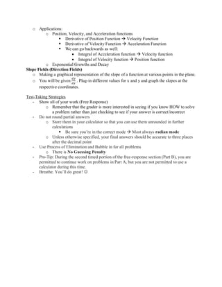
- The exam is 3 hours 15 minutes long and divided into multiple choice and free response sections testing limits, derivatives, integrals, and applications of calculus.
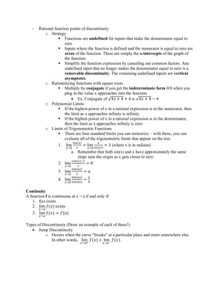
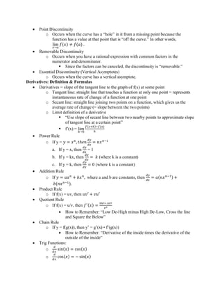
- Content topics covered include limits of functions, continuity, derivatives and their applications (related rates, max/min problems), integrals, and differential equations.
- Formulas and strategies are provided for evaluating limits, finding derivatives using various rules, applying derivatives to sketch curves, solve optimization problems, and solve motion problems using related rates.
![AP Advantage: AP Calculus AB
Classroom Matters
Instructor: Shashank Patil
May 6-7, 2017
Exam Day:
Tuesday, May 9 @ 8:00AM
Exam Structure:
Time: 3 hours 15 minutes
Section I: Multiple Choice | 45 Questions | 1 hour and 45 minutes | 50% of Final Exam Score
Part A — 30 questions | 60 minutes (calculator not permitted)
Part B — 15 questions | 45 minutes (graphing calculator required)
Section II: Free-Response | 6 Questions | 1 hour and 30 minutes | 50% of Final Exam Score
Part A — 2 problems | 30 minutes (graphing calculator required)
Part B — 4 problems | 60 minutes (calculator not permitted)
Note: You may not take both the Calculus AB and Calculus BC exams within the same year.
Content Review
Limits
• Properties of Limits:
o lim
𝑥→𝑐
(𝑓(𝑥) + 𝑔(𝑥)) = lim
𝑥→𝑎
𝑓(𝑥) + lim
𝑥→𝑎
𝑔(𝑥)
o lim
𝑥→𝑐
(𝑓(𝑥) − 𝑔(𝑥)) = lim
𝑥→𝑎
𝑓(𝑥) − lim
𝑥→𝑎
𝑔(𝑥)
o lim
𝑥→𝑐
(𝑓(𝑥)𝑔(𝑥)) = lim
𝑥→𝑎
𝑓(𝑥) × lim
𝑥→𝑎
𝑔(𝑥)
o lim
𝑥→𝑎
[𝑐𝑓(𝑥)] = c lim
𝑥→𝑎
𝑓(𝑥)
o lim
𝑥→𝑎
𝑓(𝑥)
𝑔(𝑥)
=
lim
𝑥→𝑎
𝑓(𝑥)
lim
𝑥→𝑎
𝑔(𝑥)
Finding Limits of Equations
- General: If lim
𝑥→𝑎+
𝑓(𝑥) = L and lim
𝑥→𝑎−
𝑓(𝑥) = L, then the limit lim
𝑥→𝑎
𝑓(𝑥) exists.
o If not, the limit does not exist.
- Limits by direct substitution
o F is continuous at x= a if lim
𝑥→𝑎
𝑓(𝑥) = f(a)
- Finding limits by factoring
o Find limit as x approaches 2 of f(x) = (x2
+ x – 6)/(x-2)
▪ Factor numerator and simplify to f(x) = x + 3
▪ Solution: 5
- If k and n are constants, |x| > 1, and n >0, then lim
𝑥→
𝑘
𝑥 𝑛
= 0, and lim
𝑥→ −
𝑘
𝑥 𝑛
= 0](https://image.slidesharecdn.com/apadvantage-calculusabcurriculum-170420045211/85/AP-Advantage-AP-Calculus-1-320.jpg)
![AP Advantage: AP Calculus AB
Classroom Matters
Instructor: Shashank Patil
May 6-7, 2017
Exam Day:
Tuesday, May 9 @ 8:00AM
Exam Structure:
Time: 3 hours 15 minutes
Section I: Multiple Choice | 45 Questions | 1 hour and 45 minutes | 50% of Final Exam Score
Part A — 30 questions | 60 minutes (calculator not permitted)
Part B — 15 questions | 45 minutes (graphing calculator required)
Section II: Free-Response | 6 Questions | 1 hour and 30 minutes | 50% of Final Exam Score
Part A — 2 problems | 30 minutes (graphing calculator required)
Part B — 4 problems | 60 minutes (calculator not permitted)
Note: You may not take both the Calculus AB and Calculus BC exams within the same year.
Content Review
Limits
• Properties of Limits:
o lim
𝑥→𝑐
(𝑓(𝑥) + 𝑔(𝑥)) = lim
𝑥→𝑎
𝑓(𝑥) + lim
𝑥→𝑎
𝑔(𝑥)
o lim
𝑥→𝑐
(𝑓(𝑥) − 𝑔(𝑥)) = lim
𝑥→𝑎
𝑓(𝑥) − lim
𝑥→𝑎
𝑔(𝑥)
o lim
𝑥→𝑐
(𝑓(𝑥)𝑔(𝑥)) = lim
𝑥→𝑎
𝑓(𝑥) × lim
𝑥→𝑎
𝑔(𝑥)
o lim
𝑥→𝑎
[𝑐𝑓(𝑥)] = c lim
𝑥→𝑎
𝑓(𝑥)
o lim
𝑥→𝑎
𝑓(𝑥)
𝑔(𝑥)
=
lim
𝑥→𝑎
𝑓(𝑥)
lim
𝑥→𝑎
𝑔(𝑥)
Finding Limits of Equations
- General: If lim
𝑥→𝑎+
𝑓(𝑥) = L and lim
𝑥→𝑎−
𝑓(𝑥) = L, then the limit lim
𝑥→𝑎
𝑓(𝑥) exists.
o If not, the limit does not exist.
- Limits by direct substitution
o F is continuous at x= a if lim
𝑥→𝑎
𝑓(𝑥) = f(a)
- Finding limits by factoring
o Find limit as x approaches 2 of f(x) = (x2
+ x – 6)/(x-2)
▪ Factor numerator and simplify to f(x) = x + 3
▪ Solution: 5
- If k and n are constants, |x| > 1, and n >0, then lim
𝑥→
𝑘
𝑥 𝑛
= 0, and lim
𝑥→ −
𝑘
𝑥 𝑛
= 0](https://image.slidesharecdn.com/apadvantage-calculusabcurriculum-170420045211/75/AP-Advantage-AP-Calculus-1-2048.jpg)
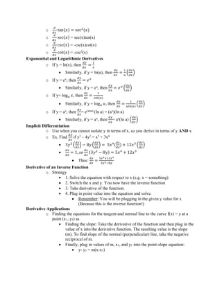
![o Mean Value Theorem for Derivatives
• If y = f(x) is continuous on the interval [a,b] and is differentiable
everywhere on the interval (a,b), then there is at least one number c
between a and b such that,
• 𝑓′(𝑐) =
𝑓(𝑏)−𝑓(𝑎)
𝑏−𝑎
• “There’s some point in the interval where the slope of the tangent
line equals the slope of the secant line that connects the endpoints
of the interval”
• Rolle’s Theorem (Special Case of MVT)
• Same as Mean Value Theorem but in this case f(a) = f(b) = 0, so
the formula simplifies to finding the value of c where f’(c) = 0
o Maxima and Minima
• A maximum or minimum of a function occurs at a point where the
derivative of the function is zero, or where the derivative fails to exist.
• Relative (local) max/min: means that the curve has a horizontal
line at that point, but it is not the highest or lowest value that the
function attains.
• Absolute (global) max/min: occurs at an end point or an x-value
where there is a vertical asymptote
• Second Derivative Test: If a function has a critical value at x = c, then that
value is relative maximum if f’’(x) < 0 and it is a relative minimum if
f’’(x) > 0
• Intuition: Let’s look at the slope of the graph of f’(x)
• Application: Knowing the maxima or minima will help us to optimize
functions
o Curve Sketching
• Find Intercepts
• Set f(x) = 0, then solve for x. This tells you the function’s x-
intercepts (or roots)
• Set x= 0 to find y-intercept(s)
• Find Asymptotes
• Horizontal Asymptotes: Find limits of f(x) as x approaches + and
-
o If they give you an interval, evaluate f(x) at the endpoints
• Vertical Asymptotes: Find values of x that make f(x) undefined
• Test the First Derivative
• Find where f’(x) = 0. This tells you the critical points
(maxima/minima).
• When f’(x) >0, the curve is rising; when f’(x) < 0, the curve is
falling.
• Test the Second Derivative
• Find where f’’(x) = 0. This tells you the inflection points.
• When f’’(x) > 0, the curve is concave up; when f’’(x) < 0, the
curve is concave down](https://image.slidesharecdn.com/apadvantage-calculusabcurriculum-170420045211/85/AP-Advantage-AP-Calculus-5-320.jpg)
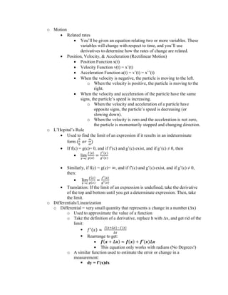
![______________________________________________________________________________
Integrals (Antiderivative)
• Used to help find area under curve or evaluate volume enclosed by a function
• Power Rule: If f(x) = xn
, then ∫ 𝑓(𝑥)𝑑𝑥 =
𝑥 𝑛+1
𝑛+1
+ 𝐶 (except when n = -1)
o It follows that:
▪ ∫ 𝑘𝑓(𝑥)𝑑𝑥 = 𝑘 ∫ 𝑓(𝑥)𝑑𝑥
▪ ∫[𝑓(𝑥) + 𝑔(𝑥)]𝑑𝑥 = ∫ 𝑓(𝑥)𝑑𝑥 + ∫ 𝑔(𝑥)𝑑𝑥
▪ ∫ 𝑘𝑑𝑥 = 𝑘𝑥 + 𝐶
• Integrals of Trig Functions
o ∫ sin(ax)𝑑𝑥 = −
cos(ax)
a
+ C
o ∫ cos(ax)𝑑𝑥 =
sin(ax)
a
+ C
o ∫ sec(ax) tan(𝑎𝑥) 𝑑𝑥 =
sec(ax)
a
+ C
o ∫ sec2
𝑎𝑥 𝑑𝑥 =
tan(ax)
a
+ C
o ∫ csc(ax) cot(𝑎𝑥) 𝑑𝑥 = −
csc(ax)
a
+ C
o ∫ csc2
𝑎𝑥 𝑑𝑥 = −
cot(ax)
a
+ C
o ∫
du
u
= ln |u| + C
o ∫ tan(x)𝑑𝑥 = −ln|cos 𝑥| + C
o ∫ cot(x)𝑑𝑥 = ln|sin 𝑥| + C
o ∫ sec(𝑥) = ln|sec(x) + tan(𝑥)| + C
o ∫ csc(x)𝑑𝑥 = −ln|csc(x) + cot(𝑥)| + C
o ∫ ex
dx =
1
k
ekx
+ C
• Integration technique: U-substitution
o ∫ un
du =
un+1
n+1
+ C
o Pick one expression to equal u, derive u, and then plug in values of u and du into
original equation.
Evaluating Integrals using Geometry
o Using Riemann Sums to estimate the integral of a function
▪ Translation: Finding area under a curve by adding up areas of rectangles
▪ Formulas (Don’t memorize these!):
• Left-Handed Sum
o
𝑏−𝑎
𝑛
(y0+ y1 + y2 + y3 + y4 + …+yn-1)
• Right-Handed Sum
o
𝑏−𝑎
𝑛
(y1 + y2 + y3 + y4 +y5 …+yn)
• Midpoint Sums
o
𝑏−𝑎
𝑛
(y1/2 + y3/2 + y5/2 + y7/2 +y9/2 …+y[2n-1]/2)
o Note: Fractional subscript means to evaluate the function at
the number half-way between each integral pair of n-values](https://image.slidesharecdn.com/apadvantage-calculusabcurriculum-170420045211/85/AP-Advantage-AP-Calculus-7-320.jpg)
![• Where a = left endpoint of the interval, b= right endpoint of the
interval, and n= number of triangles we’re using
o Trapezoid Rule = Better at estimating area than Riemann Sum method
▪ Finding area under a curve by adding up areas of trapezoids
▪ Formula
• Using formula for area of a trapezoid A= ½ (b1+ b2)(h) you can
derive the formula:
• (
1
2
) (
𝑏−𝑎
𝑛
)(y0+2y1+2y2+2y3+…+2yn-2+2yn-1+yn)
The First Fundamental Theorem of Calculus
o ∫ f(x)dx = F(b) − F(a); where F(x)is the antiderivative of f(x)
b
a
The Second Fundamental Theorem of Calculus
o If f(x) is continuous on [a,b], then the derivative of the function F(x) = ∫ 𝑓(𝑡)𝑑𝑡
𝑥
𝑎
is:
▪
dF
dx
=
𝑑
𝑑𝑥
∫ 𝑓(𝑡)𝑑𝑡 = 𝑓(𝑥)
𝑥
𝑎
• All we are concerned with is swapping the upper variable term (in
this case x) with the variable in the function (in this case t)
o The bottom term could be any constant value
• If the upper variable term is a function of x (e.g. x2
), we multiply
the answer by the derivative of that term (e.g. 2x)
Mean Value Theorem for Integrals
o Enables you to find the average value of a function
o If f(x) is continuous on a closed interval [a,b], then at some point c in the interval
[a,b] the following is true:
▪ ∫ 𝑓(𝑥)𝑑𝑥 = 𝑓(𝑐)(𝑏 − 𝑎)
𝑏
𝑎
• Translation: The area under the curve of f(x) on the interval [a,b] is
equal to the value of the function at some value c (between a and
b) times the length of the interval.
o This equation can be rearranged to find the average value of a function:
▪ 𝑓(𝑐) =
1
𝑏−𝑎
∫ 𝑓(𝑥)𝑑𝑥
𝑏
𝑎
Area Between Two Curves
o Vertical Slices
o If a region is bounded by f(x) above and g(x) below at all points of the interval
[a,b], then the area of the region is given by:
▪ ∫ [ 𝑓( 𝑥) − 𝑔( 𝑥)] 𝑑𝑥
𝑏
𝑎
o Horizontal Slices
o If a region is bounded by f(y) on the right and g(y) on the left at all points of the
interval [c,d], then the area of the region is given by
▪ ∫ [𝑓(𝑦) − 𝑔(𝑦)]𝑑𝑦
𝑑
𝑐](https://image.slidesharecdn.com/apadvantage-calculusabcurriculum-170420045211/85/AP-Advantage-AP-Calculus-8-320.jpg)
![Volume of a Solid of Revolution
o Washers (Disk) Method: Finding the volume of a complex shape by adding up volumes
of many thin discs
o Think: “You’re adding up the volume of each thin pancake in a stack!”
o Disk: If you have a region whose area is bounded by the curve y = f(x) and the x-
axis on the interval [a,b], each disk has a radius of f(x), and the area of each disk
will be π[f(x)]2
(Just like the area of a circle of a circle is A = πr2
!)
▪ To find the volume, evaluate the integral:
• π ∫ [𝑓(𝑥)]2
𝑑𝑥
𝑏
𝑎
(where dx is some small depth along the x-axis)
o Washer: If you have a region whose area is bounded above the curve y = f(x) and
below by the curve y = g(x), on the interval [a,b], then each washer will have an
area of π[f(x)2
– g(x)2
] (We’re subtracting the area of one circle from another!)
▪ To find the volume, evaluate the integral: (rotated about the x-axis)
• π ∫ [𝑓( 𝑥)2
− 𝑔( 𝑥)2
]
𝑏
𝑎
dx
▪ Finding volume for washers when the region is rotated about y –axis:
• π ∫ [𝑓(𝑦)2
− 𝑔(𝑦)2
]
𝑑
𝑐
dy
o Remember: dy and dx just stand for really (infinitesimally) small depths along the
y or x axis respectively!
o Cylindrical Shells Method
o Think: “Finding the volume of each layer of an onion” (Shrek!)
o If you have a region whose area is bounded above by the curve y= f(x) and below
by the curve y = g(x), on the interval [a,b], then each cylinder will have a height
f(x) – g(x), a radius of x, and an area of 2 πx[f(x)-g(x)].
▪ Volume when the region is rotated around the y-axis:
• 2π∫ 𝑥[𝑓(𝑥) − 𝑔(𝑥)]𝑑𝑥
𝑏
𝑎
o If you have a region whose area is bounded on the right by the curve x =f(y) and
on the left by the curve x =g(y), on the interval [c,d], then each cylinder will have
a height of f(y) – g(y), a radius of y, and an area of 2 πy[f(y)-g(y)].
▪ Volume when the region is rotated around the x-axis:
• 2𝜋 ∫ 𝑦[𝑓(𝑦) − 𝑔(𝑦)]
𝑑
𝑐
dy
o Volumes of Solids with Known Cross-Sections
o If you’re given an object where you know 1) the shape of the base and 2) that the
perpendicular cross-sections are all the same regular, planar geometric shape
▪ You can integrate using the area of that shape!
▪ Strategy: Find the area of the regular (=all sides are equal) shape, multiply
by it some small depth dy or dx (depending on how the object is oriented),
and then integrate from the endpoints of an interval
Differential Equations
o Equations that relate a function with one or more of its derivatives
o How to solve differential problems:
o Separate the variables
o Integrate both sides
o Solve for the constant](https://image.slidesharecdn.com/apadvantage-calculusabcurriculum-170420045211/85/AP-Advantage-AP-Calculus-9-320.jpg)