SlideShare a Scribd company logo
INTRODUCTORY MATHEMATICALINTRODUCTORY MATHEMATICAL
ANALYSISANALYSISFor Business, Economics, and the Life and Social Sciences
©2007 Pearson Education Asia
Chapter 17Chapter 17
Multivariable CalculusMultivariable Calculus
©2007 Pearson Education Asia
INTRODUCTORY MATHEMATICAL
ANALYSIS
0. Review of Algebra
1. Applications and More Algebra
2. Functions and Graphs
3. Lines, Parabolas, and Systems
4. Exponential and Logarithmic Functions
5. Mathematics of Finance
6. Matrix Algebra
7. Linear Programming
8. Introduction to Probability and Statistics
©2007 Pearson Education Asia
9. Additional Topics in Probability
10. Limits and Continuity
11. Differentiation
12. Additional Differentiation Topics
13. Curve Sketching
14. Integration
15. Methods and Applications of Integration
16. Continuous Random Variables
17. Multivariable Calculus
INTRODUCTORY MATHEMATICAL
ANALYSIS
©2007 Pearson Education Asia
• To discuss functions of several variables and to
compute function values.
• To compute partial derivatives.
• To develop the notions of partial marginal cost,
marginal productivity, and competitive and
complementary products.
• To find partial derivatives of a function defined
implicitly.
• To compute higher-order partial derivatives.
• To find the partial derivatives of a function by
using the chain rule.
Chapter 17: Multivariable Calculus
Chapter ObjectivesChapter Objectives
©2007 Pearson Education Asia
• To apply the second-derivative test for a
function of two variables.
• To find critical points for a function.
• To develop the method of least squares.
• To compute double and triple integrals.
Chapter 17: Multivariable Calculus
Chapter ObjectivesChapter Objectives
©2007 Pearson Education Asia
Functions of Several Variables
Partial Derivatives
Applications of Partial Derivatives
Implicit Partial Differentiation
Higher-Order Partial Derivatives
Chain Rule
Maxima and Minima for Functions of Two Variables
17.1)
17.2)
17.3)
Chapter 17: Multivariable Calculus
Chapter OutlineChapter Outline
17.4)
17.5)
17.6)
17.7)
©2007 Pearson Education Asia
Lagrange Multipliers
Lines of Regression
Multiple Integrals
17.8)
17.9)
17.10)
Chapter 17: Multivariable Calculus
Chapter OutlineChapter Outline
©2007 Pearson Education Asia
Chapter 17: Multivariable Calculus
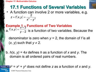
17.1 Functions of Several Variables17.1 Functions of Several Variables
Example 1 – Functions of Two Variables
• A function can involve 2 or more variables, e.g.
( ) 22
2
,
yx
yxfz
−
==
a. is a function of two variables. Because the
denominator is zero when y = 2, the domain of f is all
(x, y) such that y ≠ 2.
b. h(x, y) = 4x defines h as a function of x and y. The
domain is all ordered pairs of real numbers.
c. z2
= x2
+ y2
does not define z as a function of x and y.
( )
2
3
,
−
+
=
y
x
yxf
©2007 Pearson Education Asia
Chapter 17: Multivariable Calculus
17.1 Functions of Several Variables
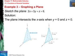
Example 3 – Graphing a Plane
Sketch the plane
Solution:
The plane intersects the x-axis when y = 0 and z = 0.
.632 =++ zyx
©2007 Pearson Education Asia
Chapter 17: Multivariable Calculus
17.1 Functions of Several Variables
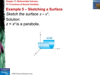
Example 5 – Sketching a Surface
Sketch the surface
Solution:
z = x2
is a parabola.
.2
xz =
©2007 Pearson Education Asia
Chapter 17: Multivariable Calculus
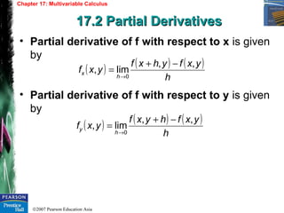
17.2 Partial Derivatives17.2 Partial Derivatives
• Partial derivative of f with respect to x is given
by
• Partial derivative of f with respect to y is given
by
( ) ( ) ( )
h
yxfyhxf
yxf
h
x
,,
lim,
0
−+
=
→
( ) ( ) ( )
h
yxfhyxf
yxf
h
y
,,
lim,
0
−+
=
→
©2007 Pearson Education Asia
Chapter 17: Multivariable Calculus
17.2 Partial Derivatives
Example 1 – Finding Partial Derivatives
If f(x, y) = xy2
+ x2
y, find fx(x, y) and fy(x, y). Also, find
fx(3, 4) and fy(3, 4).
Solution: The partial derivatives are
Thus, the solutions are
( ) ( ) ( ) xyyyxyyxfx 221, 22
+=+=
( ) ( ) ( ) 22
212, xxyxyxyxfy +=+=
( )
( ) 334,3
404,3
=
=
xy
x
f
f
©2007 Pearson Education Asia
Chapter 17: Multivariable Calculus
17.2 Partial Derivatives
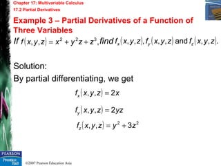
Example 3 – Partial Derivatives of a Function of
Three Variables
If find
Solution:
By partial differentiating, we get
( ) ,,, 322
zzyxzyxf ++= ( ) ( ) ( ).,,and,,,,, zyxfzyxfzyxf zyx
( ) xzyxfx 2,, =
( ) yzzyxfy 2,, =
( ) 22
3,, zyzyxfz +=
©2007 Pearson Education Asia
Chapter 17: Multivariable Calculus
17.2 Partial Derivatives
Example 4 – Finding Partial Derivatives
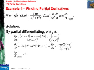
If find
Solution:
By partial differentiating, we get
( ) ,,,, 22
tsrt
rsu
utsrgp
+
==
( )
.and,
1,1,1,0t
p
t
p
s
p
∂
∂
∂
∂
∂
∂
( )( ) ( )( )
( )
( )
( )22
2
222
22
2
srtt
srtru
tsrt
strsurutsrt
s
p
+
−
=
+
−+
=
∂
∂
( ) ( ) ( )
( )222
2
2222 2
2
tsrt
srtrsu
s
p
srttsrtrsu
t
p
+
+
−=
∂
∂
⇒++−=
∂
∂ −
( )
0
1,1,1,0
=
∂
∂
t
p
©2007 Pearson Education Asia
Chapter 17: Multivariable Calculus
17.3 Applications of Partial Derivatives17.3 Applications of Partial Derivatives
Example 1 – Marginal Costs
• Interpretation of rate of change:
A company manufactures two types of skis, the Lightning and the
Alpine models. Suppose the joint-cost function for producing x pairs
of the Lightning model and y pairs of the Alpine model per week is
where c is expressed in dollars. Determine the marginal costs ∂c/∂x
and ∂c/∂y when x = 100 and y = 50, and interpret the results.
fixed.heldiswhentorespectwithofchangeofratetheis
xyz
y
z
yxz
x
z
∂
∂
∂
∂
( ) 6000857507.0, 2
+++== yxxyxfc
©2007 Pearson Education Asia
Chapter 17: Multivariable Calculus
17.3 Applications of Partial Derivatives
Example 1 – Marginal Costs
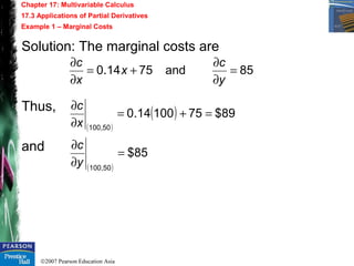
Solution: The marginal costs are
Thus,
and
( )
( )
( )
85$
89$7510014.0
50,100
50,100
=
∂
∂
=+=
∂
∂
y
c
x
c
85and7514.0 =
∂
∂
+=
∂
∂
y
c
x
x
c
©2007 Pearson Education Asia
Chapter 17: Multivariable Calculus
17.3 Applications of Partial Derivatives
Example 3 – Marginal Productivity
A manufacturer of a popular toy has determined
that the production function is P = √(lk), where l is
the number of labor-hours per week and k is the
capital (expressed in hundreds of dollars per week)
required for a weekly production of P gross of the
toy. (One gross is 144 units.) Determine the
marginal productivity functions, and evaluate them
when l = 400 and k = 16. Interpret the results.
©2007 Pearson Education Asia
Chapter 17: Multivariable Calculus
17.3 Applications of Partial Derivatives
Example 3 – Marginal Productivity
Solution: Since ,
Thus, ( )
lk
l
k
P
lk
k
klk
l
P
2
and
22
1 2/1
=
∂
∂
==
∂
∂ −
( ) 2/1
lkP =
2
5
and
10
1
16,40016,400
=
∂
∂
=
∂
∂
==== klkl k
P
l
P
©2007 Pearson Education Asia
Chapter 17: Multivariable Calculus
17.4 Implicit Partial Differentiation17.4 Implicit Partial Differentiation
Example 1 – Implicit Partial Differentiation
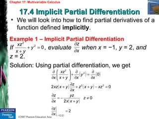
• We will look into how to find partial derivatives of a
function defined implicitly.
If , evaluate when x = −1, y = 2, and
z = 2.
Solution: Using partial differentiation, we get
02
2
=+
+
y
yx
xz
x
z
∂
∂
( ) ( )
( ) ( )
( )
0
2
02
0
22
2
2
≠
+
−=
∂
∂
=−++
∂
∂
+
∂
∂
=
∂
∂
+





+∂
∂
z
yxx
yz
x
z
xzyxz
x
z
yxxz
x
y
xyx
xz
x
( )
2
2,2,1
=
∂
∂
−x
z
©2007 Pearson Education Asia
Chapter 17: Multivariable Calculus
17.5 Higher-Order Partial Derivatives17.5 Higher-Order Partial Derivatives
Example 1 – Second-Order Partial Derivatives
• We obtain second-order partial derivatives of f
as
Find the four second-order partial derivatives of
Solution:
yyyyxyyx
yxxyxxxx
ffff
ffff
)(meansand)(means
)(meansand)(means
( ) ., 222
yxyxyxf +=
( )
( ) ( ) xyxyxfyyyxf
xyxyyxf
xyxx
x
42,and22,
22,
2
2
+=+=
+=
( )
( ) ( ) xyxyxfxyxf
yxxyxf
yxyy
y
42,and2,
2,
2
22
+==
+=
©2007 Pearson Education Asia
Chapter 17: Multivariable Calculus
17.5 Higher-Order Partial Derivatives
Example 3 – Second-Order Partial Derivative of an
Implicit Function
Determine if
Solution: By implicit differentiation,
Differentiating both sides with respect to x, we obtain
Substituting ,
2
2
x
z
∂
∂ .2
xyz =
( ) ( ) 0
2
2
≠=
∂
∂
⇒
∂
∂
=
∂
∂
z
z
y
x
z
xy
x
z
x
x
z
yz
x
z
yz
xx
z
x ∂
∂
−=
∂
∂
⇒





∂
∂
=





∂
∂
∂
∂ −− 2
2
2
1
2
1
2
1
z
y
x
z
2
=
∂
∂
0
422
1
3
2
2
2
2
≠−=





−=
∂
∂ −
z
z
y
z
y
yz
x
z
©2007 Pearson Education Asia
Chapter 17: Multivariable Calculus
17.6 Chain Rule17.6 Chain Rule
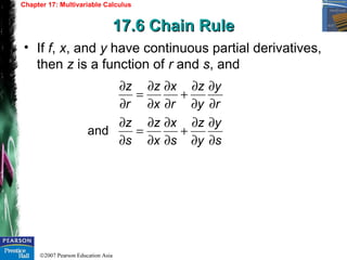
• If f, x, and y have continuous partial derivatives,
then z is a function of r and s, and
s
y
y
z
s
x
x
z
s
z
r
y
y
z
r
x
x
z
r
z
∂
∂
∂
∂
+
∂
∂
∂
∂
=
∂
∂
∂
∂
∂
∂
+
∂
∂
∂
∂
=
∂
∂
and
©2007 Pearson Education Asia
Chapter 17: Multivariable Calculus
17.6 Chain Rule
Example 1 – Rate of Change of Cost
For a manufacturer of cameras and film, the total
cost c of producing qC cameras and qF units of film is
given by
The demand functions for the cameras and film are
given by
where pC is the price per camera and pF is the price
per unit of film. Find the rate of change of total cost
with respect to the price of the camera when pC = 50
and pF = 2.
900015.030 +++= FFC qqqqcc
FCF
F
ppq
ppc
qc 4002000and
9000
−−==
©2007 Pearson Education Asia
Chapter 17: Multivariable Calculus
17.6 Chain Rule
Example 1 – Chain Rule
Example 3 – Chain Rule
Solution: By the chain rule,
Thus,
( ) ( )( )11015.0
9000
015.030 2
−++







−
+=
∂
∂
∂
∂
+
∂
∂
∂
∂
=
∂
∂
C
FC
F
C
F
FC
C
CC
q
pp
q
p
q
p
c
p
q
q
c
p
c
2.123
2,50
−≈
∂
∂
== FC ppCp
c
a. Determine ∂y/∂r if
Solution: By the chain rule,
( ) ( ) .3and6ln
642
srxxxy +=+=
( ) ( )





++
+
+=
∂
∂
∂
∂
=
∂
∂
6ln
6
2
312 4
4
4
5
x
x
x
srx
r
x
x
y
r
y
©2007 Pearson Education Asia
Chapter 17: Multivariable Calculus
17.6 Chain Rule
Example 3 – Chain Rule
b. Given that z = exy
, x = r − 4s, and y = r − s, find
∂z/∂r in terms of r and s.
Solution: By the chain rule,
Since x = r − 4s and y = r − s,
( ) xy
eyx
r
y
y
z
r
x
x
z
r
z
+=
∂
∂
∂
∂
+
∂
∂
∂
∂
=
∂
∂
( )
22
45
4
52 srsr
sry
xrx
esr
r
z +−
−=
−=
−=
∂
∂
©2007 Pearson Education Asia
Chapter 17: Multivariable Calculus
17.7 Maxima and Minima for Functions17.7 Maxima and Minima for Functions
of Two Variablesof Two Variables
• Relative maximum at the point (a, b) is shown as
RULE 1
Find relative maximum or minimum when
RULE 2 Second-Derivative Test for Functions of Two Variables
Let D be the function defined by
1. If D(a, b) > 0 and fxx(a, b) < 0, relative maximum at (a, b);
2. If D(a, b) > 0 and fxx(a, b) > 0, relative minimum at (a, b);
3. If D(a, b) < 0, then f has a saddle point at (a, b);
4. If D(a, b) = 0, no conclusion.
( ) ( )yxfbaf ,, ≥
( )
( )


=
=
0,
0,
yxf
yxf
y
x
( ) ( ) ( ) ( )( ) .,,,,
2
yxfyxfyxfyxD xyyyxx −=
©2007 Pearson Education Asia
Chapter 17: Multivariable Calculus
17.7 Maxima and Minima for Functions of Two Variables
Example 1 – Finding Critical Points
Find the critical points of the following functions.
a.
Solution:
Since
we solve the system and get
b.
Solution:
Since
we solve the system and get and
( ) 13522, 22
+−+−+= yxxyyxyxf
( ) ( ) ,0322,and0524, =−+−==+−= yxyxfyxyxf yx



=
−=
2
1
1
y
x
( ) lkklklf −+= 33
,
( ) ( ) ,03,and03, 22
=−==−= lkklfklklf kl



=
=
0
0
k
l
.
3
1
3
1



=
=
k
l
©2007 Pearson Education Asia
Chapter 17: Multivariable Calculus
17.7 Maxima and Minima for Functions of Two Variables
Example 1 – Finding Critical Points
c.
Since
we solve the system and get
( ) ( )1001002,, 22
−+−+++= yxzyxyxzyxf
( )
( )
( ) 0100,,
02,,
04,,
=+−−=
=−+=
=−+=
yxzyxf
zyxzyxf
zyxzyxf
z
y
x





=
=
=
175
75
25
z
y
x
©2007 Pearson Education Asia
Chapter 17: Multivariable Calculus
17.7 Maxima and Minima for Functions of Two Variables
Example 3 – Applying the Second-Derivative Test
Examine f(x,y) = x3
+ y3
− xy for relative maxima or
minima by using the second derivative test.
Solution: We find critical points,
which gives (0, 0) and (1/3, 1/3).
Now,
Thus,
D(0, 0) < 0  no relative extremum at (0, 0).
D(1/3,1/3)>0 and fxx(1/3,1/3)>0 relative minimum at (1/3,1/3)
Value of the function is
( ) ( ) 03,and03, 22
=−==−= xyyxfyxyxf yx
( ) ( ) ( ) 1,6,6, −=== yxfyyxfxyxf xyyyxx
( ) ( )( ) ( ) 136166,
2
−=−−= xyyxyxD
( ) ( ) ( ) ( )( ) 27
1
3
1
3
13
3
13
3
1
3
1
3
1
, −=−+=f
©2007 Pearson Education Asia
Chapter 17: Multivariable Calculus
17.7 Maxima and Minima for Functions of Two Variables
Example 5 – Finding Relative Extrema
Examine f(x, y) = x4
+ (x − y)4
for relative extrema.
Solution: We find critical points at (0,0) through
D(0, 0) = 0  no information.
f has a relative (and absolute) minimum at (0, 0).
( ) ( ) ( ) ( )
( ) ( ) ( ) ( ) ( ) 0,12,02112,
04,044,
222
333
=−==−+=
=−−==−+=
yxfyxyxfyxxyxf
yxyxfyxxyxf
xyyyxx
yx
©2007 Pearson Education Asia
Chapter 17: Multivariable Calculus
17.7 Maxima and Minima for Functions of Two Variables
Example 7 – Profit Maximization
A candy company produces two types of candy, A and
B, for which the average costs of production are
constant at $2 and $3 per pound, respectively. The
quantities qA, qB (in pounds) of A and B that can be
sold each week are given by the joint-demand
functions
where pA and pB are the selling prices (in dollars per
pound) of A and B, respectively. Determine the selling
prices that will maximize the company’s profit P.
( )
( )BAB
ABA
ppq
ppq
29400
400
−+=
−=
©2007 Pearson Education Asia
Chapter 17: Multivariable Calculus
17.7 Maxima and Minima for Functions of Two Variables
Example 7 – Profit Maximization
Solution:
The total profit is given by
The profits per pound are pA − 2 and pB − 3,
The solution is pA = 5.5 and pB = 6.
Since ∂2
P/∂p2
A< 0, we indeed have a maximum.
( ) ( )
01342and0122
32
=+−=
∂
∂
=−+−=
∂
∂
−+−=
BA
B
BA
A
BBAA
pp
p
P
pp
p
P
qpqpP
8001600800
2
2
2
2
2
=
∂∂
∂
−=
∂
∂
−=
∂
∂
ABBA pp
P
p
P
p
P
( ) 06,5.5 >D
©2007 Pearson Education Asia
Chapter 17: Multivariable Calculus
17.8 Lagrange Multipliers17.8 Lagrange Multipliers
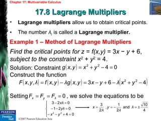
Example 1 – Method of Lagrange Multipliers
• Lagrange multipliers allow us to obtain critical points.
• The number λ0 is called a Lagrange multiplier.
Find the critical points for z = f(x,y) = 3x − y + 6,
subject to the constraint x2
+ y2
= 4.
Solution: Constraint
Construct the function
Setting , we solve the equations to be
( ) 04, 22
=−+= yxyxg
( ) ( ) ( ) ( )463,,,, 22
−+−+−=−= yxλyxyxgλyxfλyxF
0=== λyx FFF
4
10
and
2
1
,
2
3
±=−== λ
λ
y
λ
x





=+−−
=−−
=−
04
021
023
22
yx
λy
λx
©2007 Pearson Education Asia
Chapter 17: Multivariable Calculus
17.8 Lagrange Multipliers
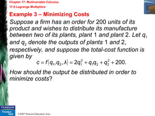
Example 3 – Minimizing Costs
Suppose a firm has an order for 200 units of its
product and wishes to distribute its manufacture
between two of its plants, plant 1 and plant 2. Let q1
and q2 denote the outputs of plants 1 and 2,
respectively, and suppose the total-cost function is
given by
How should the output be distributed in order to
minimize costs?
( ) .2002,, 2
221
2
121 +++== qqqqλqqfc
©2007 Pearson Education Asia
Chapter 17: Multivariable Calculus
17.8 Lagrange Multipliers
Example 3 – Minimizing Costs
Solution: We minimize c = f(q1, q2), given the constraint
q1 + q2 = 200.
( ) ( )2002002,, 21
2
221
2
121 −+−+++= qqλqqqqλqqF









=+−−=
∂
∂
=−+=
∂
∂
=−+=
∂
∂
0200
02
04
21
21
2
21
1
qq
λ
F
λqq
q
F
λqq
q
F
150,50 21 == qq
©2007 Pearson Education Asia
Chapter 17: Multivariable Calculus
17.8 Lagrange Multipliers
Example 5 – Least-Cost Input Combination
Find critical points for f(x, y, z) = xy+ yz, subject to the
constraints x2
+ y2
= 8 and yz = 8.
Solution:
Set
We obtain 4 critical points:
(2, 2, 4) (2,−2,−4) (−2, 2, 4) (−2,−2,−4)
( ) ( ) ( )88,,,, 2
22
121 −−−+−+= yzλyxλyzxyλλzyxF









=+−=
=+−−=
=−=
=−−+=
=−=
08
08
0
02
02
2
1
22
2
21
1
yzF
yxF
λyyF
λzλyzxF
λxyF
λ
λ
z
y
x










=
=+
=
=−−+
=
y
z
yx
λ
λzλyzx
λ
x
y
8
8
1
02
2
22
2
21
1
©2007 Pearson Education Asia
Chapter 17: Multivariable Calculus
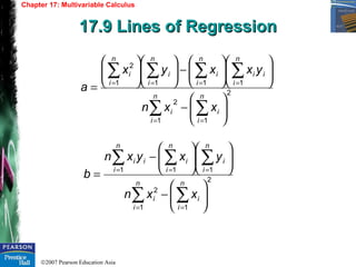
17.9 Lines of Regression17.9 Lines of Regression
2
11
2
1111
2






−












−











=
∑∑
∑∑∑∑
==
====
n
i
i
n
i
i
n
i
ii
n
i
i
n
i
i
n
i
i
xxn
yxxyx
a
2
11
2
111






−












−
=
∑∑
∑∑∑
==
===
n
i
i
n
i
i
n
i
i
n
i
ii
n
i
i
xxn
yxyxn
b
©2007 Pearson Education Asia
Chapter 17: Multivariable Calculus
17.9 Lines of Regression
Example 1 – Determining a Linear-Regression Line
By means of the linear-regression line, use the
following table to represent the trend for the index of
total U.S. government revenue from 1995 to 2000
(1995 = 100).
©2007 Pearson Education Asia
Chapter 17: Multivariable Calculus
17.9 Lines of Regression
Example 1 – Determining a Linear-Regression Line
Solution: Perform the arithmetic
( ) ( )
( ) ( )
( ) ( )
( ) ( )
83.9
21916
7362127486
3.88
21916
27482173691
2
2
≈
−
−
=
≈
−
−
=
b
a
xy 83.93.88ˆ +=
©2007 Pearson Education Asia
Chapter 17: Multivariable Calculus
17.10 Multiple Integrals17.10 Multiple Integrals
Example 1 – Evaluating a Double Integral
• Definite integrals of functions of two variables are
called (definite) double integrals, which involve
integration over a region in the plane.
Find
Solution:
( ) .12
1
1
1
0
dxdyx
x
∫ ∫−
−
+
( )
[ ]
3
2
23
2
2
12
1
1
231
1
1
0
1
1
1
0
=





++−=+=
+
−−
−
−
−
∫
∫ ∫
x
xx
dxyxy
dxdyx
x
x
©2007 Pearson Education Asia
Chapter 17: Multivariable Calculus
17.10 Lines of Regression
Example 3 – Evaluating a Triple Integral
Find
Solution:
.
1
0 0 0
dxdydzx
x yx
∫∫ ∫
−
[ ]
8
1
82
1
0
41
0 0
2
2
1
0 0
0
1
0 0 0
=





=





−=
=
∫
∫∫∫∫ ∫
−
−
x
dx
xy
yx
dxdyxzdxdydzx
x
x
yx
x yx

More Related Content

What's hot

Ordinary differential equations
Ordinary differential equationsOrdinary differential equations
Ordinary differential equations
Ahmed Haider
 
Vector calculus
Vector calculusVector calculus
Vector calculus
Kumar
 
Differential equations
Differential equationsDifferential equations
Differential equations
Charan Kumar
 
First order linear differential equation
First order linear differential equationFirst order linear differential equation
First order linear differential equation
Nofal Umair
 

What's hot (20)

Application of derivatives
Application of derivatives Application of derivatives
Application of derivatives
 
Application of derivative
Application of derivativeApplication of derivative
Application of derivative
 
Ordinary differential equation
Ordinary differential equationOrdinary differential equation
Ordinary differential equation
 
Partial Derivatives
Partial DerivativesPartial Derivatives
Partial Derivatives
 
Integral calculus
Integral calculusIntegral calculus
Integral calculus
 
Complex analysis
Complex analysisComplex analysis
Complex analysis
 
Integration presentation
Integration presentationIntegration presentation
Integration presentation
 
Application of derivatives 2 maxima and minima
Application of derivatives 2  maxima and minimaApplication of derivatives 2  maxima and minima
Application of derivatives 2 maxima and minima
 
INTEGRATION BY PARTS PPT
INTEGRATION BY PARTS PPT INTEGRATION BY PARTS PPT
INTEGRATION BY PARTS PPT
 
limits and continuity
limits and continuity limits and continuity
limits and continuity
 
Ordinary differential equations
Ordinary differential equationsOrdinary differential equations
Ordinary differential equations
 
Differential Equations
Differential EquationsDifferential Equations
Differential Equations
 
1551 limits and continuity
1551 limits and continuity1551 limits and continuity
1551 limits and continuity
 
Partial Differential Equation - Notes
Partial Differential Equation - NotesPartial Differential Equation - Notes
Partial Differential Equation - Notes
 
Integral Calculus
Integral CalculusIntegral Calculus
Integral Calculus
 
Lesson 5: Continuity (slides)
Lesson 5: Continuity (slides)Lesson 5: Continuity (slides)
Lesson 5: Continuity (slides)
 
Vector calculus
Vector calculusVector calculus
Vector calculus
 
Applied Calculus Chapter 3 partial derivatives
Applied Calculus Chapter  3 partial derivativesApplied Calculus Chapter  3 partial derivatives
Applied Calculus Chapter 3 partial derivatives
 
Differential equations
Differential equationsDifferential equations
Differential equations
 
First order linear differential equation
First order linear differential equationFirst order linear differential equation
First order linear differential equation
 

Viewers also liked

Multivariable calculus slides 2
Multivariable calculus slides 2Multivariable calculus slides 2
Multivariable calculus slides 2
António Carneiro
 
Basic trigonometry
Basic trigonometryBasic trigonometry
Basic trigonometry
ristovanatoa
 
Mark A. McGinley curriculum vitae
Mark A. McGinley  curriculum vitaeMark A. McGinley  curriculum vitae
Mark A. McGinley curriculum vitae
Mark McGinley
 
McGinley, Temme, and Geber 1989
McGinley, Temme, and Geber 1989McGinley, Temme, and Geber 1989
McGinley, Temme, and Geber 1989
Mark McGinley
 

Viewers also liked (20)

Chapter 2 - Functions and Graphs
Chapter 2 - Functions and GraphsChapter 2 - Functions and Graphs
Chapter 2 - Functions and Graphs
 
Chapter 16 - Continuous Random Variables
Chapter 16 - Continuous Random VariablesChapter 16 - Continuous Random Variables
Chapter 16 - Continuous Random Variables
 
Chapter 3 - Lines , Parabolas and Systems
Chapter 3 - Lines , Parabolas and SystemsChapter 3 - Lines , Parabolas and Systems
Chapter 3 - Lines , Parabolas and Systems
 
Chapter 1 - Applications and More Algebra
Chapter 1 - Applications and More AlgebraChapter 1 - Applications and More Algebra
Chapter 1 - Applications and More Algebra
 
Chapter 15 - Methods and Applications of Integration
Chapter 15 - Methods and Applications of IntegrationChapter 15 - Methods and Applications of Integration
Chapter 15 - Methods and Applications of Integration
 
Chapter 6 - Matrix Algebra
Chapter 6 - Matrix AlgebraChapter 6 - Matrix Algebra
Chapter 6 - Matrix Algebra
 
Chapter 5 - Mathematics of Finance
Chapter 5 - Mathematics of FinanceChapter 5 - Mathematics of Finance
Chapter 5 - Mathematics of Finance
 
Chapter 4 - Exponential and Logarithmic Functions
Chapter 4 - Exponential and Logarithmic FunctionsChapter 4 - Exponential and Logarithmic Functions
Chapter 4 - Exponential and Logarithmic Functions
 
Chapter 7 - Linear Programming
Chapter 7 - Linear ProgrammingChapter 7 - Linear Programming
Chapter 7 - Linear Programming
 
Multivariable calculus slides 2
Multivariable calculus slides 2Multivariable calculus slides 2
Multivariable calculus slides 2
 
Matrix algebra
Matrix algebraMatrix algebra
Matrix algebra
 
Introductory maths analysis chapter 10 official
Introductory maths analysis   chapter 10 officialIntroductory maths analysis   chapter 10 official
Introductory maths analysis chapter 10 official
 
Basic trigonometry
Basic trigonometryBasic trigonometry
Basic trigonometry
 
Chapter 14 - Integration
Chapter 14 - IntegrationChapter 14 - Integration
Chapter 14 - Integration
 
Chapter 9 - Additional Topics in Probability
Chapter 9 - Additional Topics in ProbabilityChapter 9 - Additional Topics in Probability
Chapter 9 - Additional Topics in Probability
 
Chapter 13 - Curve Sketching
Chapter 13 - Curve SketchingChapter 13 - Curve Sketching
Chapter 13 - Curve Sketching
 
Woodrat Paper
Woodrat PaperWoodrat Paper
Woodrat Paper
 
Mark A. McGinley curriculum vitae
Mark A. McGinley  curriculum vitaeMark A. McGinley  curriculum vitae
Mark A. McGinley curriculum vitae
 
McGinley, Temme, and Geber 1989
McGinley, Temme, and Geber 1989McGinley, Temme, and Geber 1989
McGinley, Temme, and Geber 1989
 
Mark McGinley Story
Mark McGinley StoryMark McGinley Story
Mark McGinley Story
 

Similar to Chapter 17 - Multivariable Calculus

derivativesanditssimpleapplications-160828144729.pptx
derivativesanditssimpleapplications-160828144729.pptxderivativesanditssimpleapplications-160828144729.pptx
derivativesanditssimpleapplications-160828144729.pptx
SnehSinha6
 

Similar to Chapter 17 - Multivariable Calculus (20)

Introductory maths analysis chapter 14 official
Introductory maths analysis   chapter 14 officialIntroductory maths analysis   chapter 14 official
Introductory maths analysis chapter 14 official
 
Chapter14 integration-151007043436-lva1-app6892
Chapter14 integration-151007043436-lva1-app6892Chapter14 integration-151007043436-lva1-app6892
Chapter14 integration-151007043436-lva1-app6892
 
Chapter 12 - Additional Differentiation Topics
Chapter 12 - Additional Differentiation TopicsChapter 12 - Additional Differentiation Topics
Chapter 12 - Additional Differentiation Topics
 
Introductory maths analysis chapter 12 official
Introductory maths analysis   chapter 12 officialIntroductory maths analysis   chapter 12 official
Introductory maths analysis chapter 12 official
 
Chapter12 additionaldifferentiationtopics-151003154510-lva1-app6891
Chapter12 additionaldifferentiationtopics-151003154510-lva1-app6891Chapter12 additionaldifferentiationtopics-151003154510-lva1-app6891
Chapter12 additionaldifferentiationtopics-151003154510-lva1-app6891
 
Introductory maths analysis chapter 11 official
Introductory maths analysis   chapter 11 officialIntroductory maths analysis   chapter 11 official
Introductory maths analysis chapter 11 official
 
Chapter 11 - Differentiation
Chapter 11 - DifferentiationChapter 11 - Differentiation
Chapter 11 - Differentiation
 
Chapter11 differentiation-151003160732-lva1-app6891
Chapter11 differentiation-151003160732-lva1-app6891Chapter11 differentiation-151003160732-lva1-app6891
Chapter11 differentiation-151003160732-lva1-app6891
 
Chapter0 reviewofalgebra-151003150137-lva1-app6891
Chapter0 reviewofalgebra-151003150137-lva1-app6891Chapter0 reviewofalgebra-151003150137-lva1-app6891
Chapter0 reviewofalgebra-151003150137-lva1-app6891
 
Introductory maths analysis chapter 00 official
Introductory maths analysis   chapter 00 officialIntroductory maths analysis   chapter 00 official
Introductory maths analysis chapter 00 official
 
Introductory maths analysis chapter 02 official
Introductory maths analysis   chapter 02 officialIntroductory maths analysis   chapter 02 official
Introductory maths analysis chapter 02 official
 
Chapter2 functionsandgraphs-151003144959-lva1-app6891
Chapter2 functionsandgraphs-151003144959-lva1-app6891Chapter2 functionsandgraphs-151003144959-lva1-app6891
Chapter2 functionsandgraphs-151003144959-lva1-app6891
 
A Parallel Branch And Bound Algorithm For The Quadratic Assignment Problem
A Parallel Branch And Bound Algorithm For The Quadratic Assignment ProblemA Parallel Branch And Bound Algorithm For The Quadratic Assignment Problem
A Parallel Branch And Bound Algorithm For The Quadratic Assignment Problem
 
Chapter 10 - Limit and Continuity
Chapter 10 - Limit and ContinuityChapter 10 - Limit and Continuity
Chapter 10 - Limit and Continuity
 
Chapter10 limitandcontinuity-151003153921-lva1-app6891
Chapter10 limitandcontinuity-151003153921-lva1-app6891Chapter10 limitandcontinuity-151003153921-lva1-app6891
Chapter10 limitandcontinuity-151003153921-lva1-app6891
 
Chapter16 continuousrandomvariables-151007043951-lva1-app6892
Chapter16 continuousrandomvariables-151007043951-lva1-app6892Chapter16 continuousrandomvariables-151007043951-lva1-app6892
Chapter16 continuousrandomvariables-151007043951-lva1-app6892
 
Introductory maths analysis chapter 16 official
Introductory maths analysis   chapter 16 officialIntroductory maths analysis   chapter 16 official
Introductory maths analysis chapter 16 official
 
Derivatives and it’s simple applications
Derivatives and it’s simple applicationsDerivatives and it’s simple applications
Derivatives and it’s simple applications
 
derivativesanditssimpleapplications-160828144729.pptx
derivativesanditssimpleapplications-160828144729.pptxderivativesanditssimpleapplications-160828144729.pptx
derivativesanditssimpleapplications-160828144729.pptx
 
AIOU Code 803 Mathematics for Economists Semester Spring 2022 Assignment 2.pptx
AIOU Code 803 Mathematics for Economists Semester Spring 2022 Assignment 2.pptxAIOU Code 803 Mathematics for Economists Semester Spring 2022 Assignment 2.pptx
AIOU Code 803 Mathematics for Economists Semester Spring 2022 Assignment 2.pptx
 

Recently uploaded

anas about venice for grade 6f about venice
anas about venice for grade 6f about veniceanas about venice for grade 6f about venice
anas about venice for grade 6f about venice
anasabutalha2013
 
chapter 10 - excise tax of transfer and business taxation
chapter 10 - excise tax of transfer and business taxationchapter 10 - excise tax of transfer and business taxation
chapter 10 - excise tax of transfer and business taxation
AUDIJEAngelo
 

Recently uploaded (20)

April 2024 Nostalgia Products Newsletter
April 2024 Nostalgia Products NewsletterApril 2024 Nostalgia Products Newsletter
April 2024 Nostalgia Products Newsletter
 
Unveiling the Dynamic Gemini_ Personality Traits and Sign Dates.pptx
Unveiling the Dynamic Gemini_ Personality Traits and Sign Dates.pptxUnveiling the Dynamic Gemini_ Personality Traits and Sign Dates.pptx
Unveiling the Dynamic Gemini_ Personality Traits and Sign Dates.pptx
 
Vendors of country report usefull datass
Vendors of country report usefull datassVendors of country report usefull datass
Vendors of country report usefull datass
 
Hyundai capital 2024 1quarter Earnings release
Hyundai capital 2024 1quarter Earnings releaseHyundai capital 2024 1quarter Earnings release
Hyundai capital 2024 1quarter Earnings release
 
anas about venice for grade 6f about venice
anas about venice for grade 6f about veniceanas about venice for grade 6f about venice
anas about venice for grade 6f about venice
 
chapter 10 - excise tax of transfer and business taxation
chapter 10 - excise tax of transfer and business taxationchapter 10 - excise tax of transfer and business taxation
chapter 10 - excise tax of transfer and business taxation
 
Cracking the Change Management Code Main New.pptx
Cracking the Change Management Code Main New.pptxCracking the Change Management Code Main New.pptx
Cracking the Change Management Code Main New.pptx
 
RMD24 | Debunking the non-endemic revenue myth Marvin Vacquier Droop | First ...
RMD24 | Debunking the non-endemic revenue myth Marvin Vacquier Droop | First ...RMD24 | Debunking the non-endemic revenue myth Marvin Vacquier Droop | First ...
RMD24 | Debunking the non-endemic revenue myth Marvin Vacquier Droop | First ...
 
Falcon Invoice Discounting Setup for Small Businesses
Falcon Invoice Discounting Setup for Small BusinessesFalcon Invoice Discounting Setup for Small Businesses
Falcon Invoice Discounting Setup for Small Businesses
 
Understanding UAE Labour Law: Key Points for Employers and Employees
Understanding UAE Labour Law: Key Points for Employers and EmployeesUnderstanding UAE Labour Law: Key Points for Employers and Employees
Understanding UAE Labour Law: Key Points for Employers and Employees
 
Did Paul Haggis Ever Win an Oscar for Best Filmmaker
Did Paul Haggis Ever Win an Oscar for Best FilmmakerDid Paul Haggis Ever Win an Oscar for Best Filmmaker
Did Paul Haggis Ever Win an Oscar for Best Filmmaker
 
Byrd & Chen’s Canadian Tax Principles 2023-2024 Edition 1st edition Volumes I...
Byrd & Chen’s Canadian Tax Principles 2023-2024 Edition 1st edition Volumes I...Byrd & Chen’s Canadian Tax Principles 2023-2024 Edition 1st edition Volumes I...
Byrd & Chen’s Canadian Tax Principles 2023-2024 Edition 1st edition Volumes I...
 
Global Interconnection Group Joint Venture[960] (1).pdf
Global Interconnection Group Joint Venture[960] (1).pdfGlobal Interconnection Group Joint Venture[960] (1).pdf
Global Interconnection Group Joint Venture[960] (1).pdf
 
The Leading Cyber Security Entrepreneur of India in 2024.pdf
The Leading Cyber Security Entrepreneur of India in 2024.pdfThe Leading Cyber Security Entrepreneur of India in 2024.pdf
The Leading Cyber Security Entrepreneur of India in 2024.pdf
 
LinkedIn Masterclass Techweek 2024 v4.1.pptx
LinkedIn Masterclass Techweek 2024 v4.1.pptxLinkedIn Masterclass Techweek 2024 v4.1.pptx
LinkedIn Masterclass Techweek 2024 v4.1.pptx
 
How to Maintain Healthy Life style.pptx
How to Maintain  Healthy Life style.pptxHow to Maintain  Healthy Life style.pptx
How to Maintain Healthy Life style.pptx
 
Using Generative AI for Content Marketing
Using Generative AI for Content MarketingUsing Generative AI for Content Marketing
Using Generative AI for Content Marketing
 
12 Conversion Rate Optimization Strategies for Ecommerce Websites.pdf
12 Conversion Rate Optimization Strategies for Ecommerce Websites.pdf12 Conversion Rate Optimization Strategies for Ecommerce Websites.pdf
12 Conversion Rate Optimization Strategies for Ecommerce Websites.pdf
 
The Inspiring Personality To Watch In 2024.pdf
The Inspiring Personality To Watch In 2024.pdfThe Inspiring Personality To Watch In 2024.pdf
The Inspiring Personality To Watch In 2024.pdf
 
New Product Development.kjiy7ggbfdsddggo9lo
New Product Development.kjiy7ggbfdsddggo9loNew Product Development.kjiy7ggbfdsddggo9lo
New Product Development.kjiy7ggbfdsddggo9lo
 

Chapter 17 - Multivariable Calculus

  • 1. INTRODUCTORY MATHEMATICALINTRODUCTORY MATHEMATICAL ANALYSISANALYSISFor Business, Economics, and the Life and Social Sciences ©2007 Pearson Education Asia Chapter 17Chapter 17 Multivariable CalculusMultivariable Calculus
  • 2. ©2007 Pearson Education Asia INTRODUCTORY MATHEMATICAL ANALYSIS 0. Review of Algebra 1. Applications and More Algebra 2. Functions and Graphs 3. Lines, Parabolas, and Systems 4. Exponential and Logarithmic Functions 5. Mathematics of Finance 6. Matrix Algebra 7. Linear Programming 8. Introduction to Probability and Statistics
  • 3. ©2007 Pearson Education Asia 9. Additional Topics in Probability 10. Limits and Continuity 11. Differentiation 12. Additional Differentiation Topics 13. Curve Sketching 14. Integration 15. Methods and Applications of Integration 16. Continuous Random Variables 17. Multivariable Calculus INTRODUCTORY MATHEMATICAL ANALYSIS
  • 4. ©2007 Pearson Education Asia • To discuss functions of several variables and to compute function values. • To compute partial derivatives. • To develop the notions of partial marginal cost, marginal productivity, and competitive and complementary products. • To find partial derivatives of a function defined implicitly. • To compute higher-order partial derivatives. • To find the partial derivatives of a function by using the chain rule. Chapter 17: Multivariable Calculus Chapter ObjectivesChapter Objectives
  • 5. ©2007 Pearson Education Asia • To apply the second-derivative test for a function of two variables. • To find critical points for a function. • To develop the method of least squares. • To compute double and triple integrals. Chapter 17: Multivariable Calculus Chapter ObjectivesChapter Objectives
  • 6. ©2007 Pearson Education Asia Functions of Several Variables Partial Derivatives Applications of Partial Derivatives Implicit Partial Differentiation Higher-Order Partial Derivatives Chain Rule Maxima and Minima for Functions of Two Variables 17.1) 17.2) 17.3) Chapter 17: Multivariable Calculus Chapter OutlineChapter Outline 17.4) 17.5) 17.6) 17.7)
  • 7. ©2007 Pearson Education Asia Lagrange Multipliers Lines of Regression Multiple Integrals 17.8) 17.9) 17.10) Chapter 17: Multivariable Calculus Chapter OutlineChapter Outline
  • 8. ©2007 Pearson Education Asia Chapter 17: Multivariable Calculus 17.1 Functions of Several Variables17.1 Functions of Several Variables Example 1 – Functions of Two Variables • A function can involve 2 or more variables, e.g. ( ) 22 2 , yx yxfz − == a. is a function of two variables. Because the denominator is zero when y = 2, the domain of f is all (x, y) such that y ≠ 2. b. h(x, y) = 4x defines h as a function of x and y. The domain is all ordered pairs of real numbers. c. z2 = x2 + y2 does not define z as a function of x and y. ( ) 2 3 , − + = y x yxf
  • 9. ©2007 Pearson Education Asia Chapter 17: Multivariable Calculus 17.1 Functions of Several Variables Example 3 – Graphing a Plane Sketch the plane Solution: The plane intersects the x-axis when y = 0 and z = 0. .632 =++ zyx
  • 10. ©2007 Pearson Education Asia Chapter 17: Multivariable Calculus 17.1 Functions of Several Variables Example 5 – Sketching a Surface Sketch the surface Solution: z = x2 is a parabola. .2 xz =
  • 11. ©2007 Pearson Education Asia Chapter 17: Multivariable Calculus 17.2 Partial Derivatives17.2 Partial Derivatives • Partial derivative of f with respect to x is given by • Partial derivative of f with respect to y is given by ( ) ( ) ( ) h yxfyhxf yxf h x ,, lim, 0 −+ = → ( ) ( ) ( ) h yxfhyxf yxf h y ,, lim, 0 −+ = →
  • 12. ©2007 Pearson Education Asia Chapter 17: Multivariable Calculus 17.2 Partial Derivatives Example 1 – Finding Partial Derivatives If f(x, y) = xy2 + x2 y, find fx(x, y) and fy(x, y). Also, find fx(3, 4) and fy(3, 4). Solution: The partial derivatives are Thus, the solutions are ( ) ( ) ( ) xyyyxyyxfx 221, 22 +=+= ( ) ( ) ( ) 22 212, xxyxyxyxfy +=+= ( ) ( ) 334,3 404,3 = = xy x f f
  • 13. ©2007 Pearson Education Asia Chapter 17: Multivariable Calculus 17.2 Partial Derivatives Example 3 – Partial Derivatives of a Function of Three Variables If find Solution: By partial differentiating, we get ( ) ,,, 322 zzyxzyxf ++= ( ) ( ) ( ).,,and,,,,, zyxfzyxfzyxf zyx ( ) xzyxfx 2,, = ( ) yzzyxfy 2,, = ( ) 22 3,, zyzyxfz +=
  • 14. ©2007 Pearson Education Asia Chapter 17: Multivariable Calculus 17.2 Partial Derivatives Example 4 – Finding Partial Derivatives If find Solution: By partial differentiating, we get ( ) ,,,, 22 tsrt rsu utsrgp + == ( ) .and, 1,1,1,0t p t p s p ∂ ∂ ∂ ∂ ∂ ∂ ( )( ) ( )( ) ( ) ( ) ( )22 2 222 22 2 srtt srtru tsrt strsurutsrt s p + − = + −+ = ∂ ∂ ( ) ( ) ( ) ( )222 2 2222 2 2 tsrt srtrsu s p srttsrtrsu t p + + −= ∂ ∂ ⇒++−= ∂ ∂ − ( ) 0 1,1,1,0 = ∂ ∂ t p
  • 15. ©2007 Pearson Education Asia Chapter 17: Multivariable Calculus 17.3 Applications of Partial Derivatives17.3 Applications of Partial Derivatives Example 1 – Marginal Costs • Interpretation of rate of change: A company manufactures two types of skis, the Lightning and the Alpine models. Suppose the joint-cost function for producing x pairs of the Lightning model and y pairs of the Alpine model per week is where c is expressed in dollars. Determine the marginal costs ∂c/∂x and ∂c/∂y when x = 100 and y = 50, and interpret the results. fixed.heldiswhentorespectwithofchangeofratetheis fixed.heldiswhentorespectwithofchangeofratetheis xyz y z yxz x z ∂ ∂ ∂ ∂ ( ) 6000857507.0, 2 +++== yxxyxfc
  • 16. ©2007 Pearson Education Asia Chapter 17: Multivariable Calculus 17.3 Applications of Partial Derivatives Example 1 – Marginal Costs Solution: The marginal costs are Thus, and ( ) ( ) ( ) 85$ 89$7510014.0 50,100 50,100 = ∂ ∂ =+= ∂ ∂ y c x c 85and7514.0 = ∂ ∂ += ∂ ∂ y c x x c
  • 17. ©2007 Pearson Education Asia Chapter 17: Multivariable Calculus 17.3 Applications of Partial Derivatives Example 3 – Marginal Productivity A manufacturer of a popular toy has determined that the production function is P = √(lk), where l is the number of labor-hours per week and k is the capital (expressed in hundreds of dollars per week) required for a weekly production of P gross of the toy. (One gross is 144 units.) Determine the marginal productivity functions, and evaluate them when l = 400 and k = 16. Interpret the results.
  • 18. ©2007 Pearson Education Asia Chapter 17: Multivariable Calculus 17.3 Applications of Partial Derivatives Example 3 – Marginal Productivity Solution: Since , Thus, ( ) lk l k P lk k klk l P 2 and 22 1 2/1 = ∂ ∂ == ∂ ∂ − ( ) 2/1 lkP = 2 5 and 10 1 16,40016,400 = ∂ ∂ = ∂ ∂ ==== klkl k P l P
  • 19. ©2007 Pearson Education Asia Chapter 17: Multivariable Calculus 17.4 Implicit Partial Differentiation17.4 Implicit Partial Differentiation Example 1 – Implicit Partial Differentiation • We will look into how to find partial derivatives of a function defined implicitly. If , evaluate when x = −1, y = 2, and z = 2. Solution: Using partial differentiation, we get 02 2 =+ + y yx xz x z ∂ ∂ ( ) ( ) ( ) ( ) ( ) 0 2 02 0 22 2 2 ≠ + −= ∂ ∂ =−++ ∂ ∂ + ∂ ∂ = ∂ ∂ +      +∂ ∂ z yxx yz x z xzyxz x z yxxz x y xyx xz x ( ) 2 2,2,1 = ∂ ∂ −x z
  • 20. ©2007 Pearson Education Asia Chapter 17: Multivariable Calculus 17.5 Higher-Order Partial Derivatives17.5 Higher-Order Partial Derivatives Example 1 – Second-Order Partial Derivatives • We obtain second-order partial derivatives of f as Find the four second-order partial derivatives of Solution: yyyyxyyx yxxyxxxx ffff ffff )(meansand)(means )(meansand)(means ( ) ., 222 yxyxyxf += ( ) ( ) ( ) xyxyxfyyyxf xyxyyxf xyxx x 42,and22, 22, 2 2 +=+= += ( ) ( ) ( ) xyxyxfxyxf yxxyxf yxyy y 42,and2, 2, 2 22 +== +=
  • 21. ©2007 Pearson Education Asia Chapter 17: Multivariable Calculus 17.5 Higher-Order Partial Derivatives Example 3 – Second-Order Partial Derivative of an Implicit Function Determine if Solution: By implicit differentiation, Differentiating both sides with respect to x, we obtain Substituting , 2 2 x z ∂ ∂ .2 xyz = ( ) ( ) 0 2 2 ≠= ∂ ∂ ⇒ ∂ ∂ = ∂ ∂ z z y x z xy x z x x z yz x z yz xx z x ∂ ∂ −= ∂ ∂ ⇒      ∂ ∂ =      ∂ ∂ ∂ ∂ −− 2 2 2 1 2 1 2 1 z y x z 2 = ∂ ∂ 0 422 1 3 2 2 2 2 ≠−=      −= ∂ ∂ − z z y z y yz x z
  • 22. ©2007 Pearson Education Asia Chapter 17: Multivariable Calculus 17.6 Chain Rule17.6 Chain Rule • If f, x, and y have continuous partial derivatives, then z is a function of r and s, and s y y z s x x z s z r y y z r x x z r z ∂ ∂ ∂ ∂ + ∂ ∂ ∂ ∂ = ∂ ∂ ∂ ∂ ∂ ∂ + ∂ ∂ ∂ ∂ = ∂ ∂ and
  • 23. ©2007 Pearson Education Asia Chapter 17: Multivariable Calculus 17.6 Chain Rule Example 1 – Rate of Change of Cost For a manufacturer of cameras and film, the total cost c of producing qC cameras and qF units of film is given by The demand functions for the cameras and film are given by where pC is the price per camera and pF is the price per unit of film. Find the rate of change of total cost with respect to the price of the camera when pC = 50 and pF = 2. 900015.030 +++= FFC qqqqcc FCF F ppq ppc qc 4002000and 9000 −−==
  • 24. ©2007 Pearson Education Asia Chapter 17: Multivariable Calculus 17.6 Chain Rule Example 1 – Chain Rule Example 3 – Chain Rule Solution: By the chain rule, Thus, ( ) ( )( )11015.0 9000 015.030 2 −++        − += ∂ ∂ ∂ ∂ + ∂ ∂ ∂ ∂ = ∂ ∂ C FC F C F FC C CC q pp q p q p c p q q c p c 2.123 2,50 −≈ ∂ ∂ == FC ppCp c a. Determine ∂y/∂r if Solution: By the chain rule, ( ) ( ) .3and6ln 642 srxxxy +=+= ( ) ( )      ++ + += ∂ ∂ ∂ ∂ = ∂ ∂ 6ln 6 2 312 4 4 4 5 x x x srx r x x y r y
  • 25. ©2007 Pearson Education Asia Chapter 17: Multivariable Calculus 17.6 Chain Rule Example 3 – Chain Rule b. Given that z = exy , x = r − 4s, and y = r − s, find ∂z/∂r in terms of r and s. Solution: By the chain rule, Since x = r − 4s and y = r − s, ( ) xy eyx r y y z r x x z r z += ∂ ∂ ∂ ∂ + ∂ ∂ ∂ ∂ = ∂ ∂ ( ) 22 45 4 52 srsr sry xrx esr r z +− −= −= −= ∂ ∂
  • 26. ©2007 Pearson Education Asia Chapter 17: Multivariable Calculus 17.7 Maxima and Minima for Functions17.7 Maxima and Minima for Functions of Two Variablesof Two Variables • Relative maximum at the point (a, b) is shown as RULE 1 Find relative maximum or minimum when RULE 2 Second-Derivative Test for Functions of Two Variables Let D be the function defined by 1. If D(a, b) > 0 and fxx(a, b) < 0, relative maximum at (a, b); 2. If D(a, b) > 0 and fxx(a, b) > 0, relative minimum at (a, b); 3. If D(a, b) < 0, then f has a saddle point at (a, b); 4. If D(a, b) = 0, no conclusion. ( ) ( )yxfbaf ,, ≥ ( ) ( )   = = 0, 0, yxf yxf y x ( ) ( ) ( ) ( )( ) .,,,, 2 yxfyxfyxfyxD xyyyxx −=
  • 27. ©2007 Pearson Education Asia Chapter 17: Multivariable Calculus 17.7 Maxima and Minima for Functions of Two Variables Example 1 – Finding Critical Points Find the critical points of the following functions. a. Solution: Since we solve the system and get b. Solution: Since we solve the system and get and ( ) 13522, 22 +−+−+= yxxyyxyxf ( ) ( ) ,0322,and0524, =−+−==+−= yxyxfyxyxf yx    = −= 2 1 1 y x ( ) lkklklf −+= 33 , ( ) ( ) ,03,and03, 22 =−==−= lkklfklklf kl    = = 0 0 k l . 3 1 3 1    = = k l
  • 28. ©2007 Pearson Education Asia Chapter 17: Multivariable Calculus 17.7 Maxima and Minima for Functions of Two Variables Example 1 – Finding Critical Points c. Since we solve the system and get ( ) ( )1001002,, 22 −+−+++= yxzyxyxzyxf ( ) ( ) ( ) 0100,, 02,, 04,, =+−−= =−+= =−+= yxzyxf zyxzyxf zyxzyxf z y x      = = = 175 75 25 z y x
  • 29. ©2007 Pearson Education Asia Chapter 17: Multivariable Calculus 17.7 Maxima and Minima for Functions of Two Variables Example 3 – Applying the Second-Derivative Test Examine f(x,y) = x3 + y3 − xy for relative maxima or minima by using the second derivative test. Solution: We find critical points, which gives (0, 0) and (1/3, 1/3). Now, Thus, D(0, 0) < 0  no relative extremum at (0, 0). D(1/3,1/3)>0 and fxx(1/3,1/3)>0 relative minimum at (1/3,1/3) Value of the function is ( ) ( ) 03,and03, 22 =−==−= xyyxfyxyxf yx ( ) ( ) ( ) 1,6,6, −=== yxfyyxfxyxf xyyyxx ( ) ( )( ) ( ) 136166, 2 −=−−= xyyxyxD ( ) ( ) ( ) ( )( ) 27 1 3 1 3 13 3 13 3 1 3 1 3 1 , −=−+=f
  • 30. ©2007 Pearson Education Asia Chapter 17: Multivariable Calculus 17.7 Maxima and Minima for Functions of Two Variables Example 5 – Finding Relative Extrema Examine f(x, y) = x4 + (x − y)4 for relative extrema. Solution: We find critical points at (0,0) through D(0, 0) = 0  no information. f has a relative (and absolute) minimum at (0, 0). ( ) ( ) ( ) ( ) ( ) ( ) ( ) ( ) ( ) 0,12,02112, 04,044, 222 333 =−==−+= =−−==−+= yxfyxyxfyxxyxf yxyxfyxxyxf xyyyxx yx
  • 31. ©2007 Pearson Education Asia Chapter 17: Multivariable Calculus 17.7 Maxima and Minima for Functions of Two Variables Example 7 – Profit Maximization A candy company produces two types of candy, A and B, for which the average costs of production are constant at $2 and $3 per pound, respectively. The quantities qA, qB (in pounds) of A and B that can be sold each week are given by the joint-demand functions where pA and pB are the selling prices (in dollars per pound) of A and B, respectively. Determine the selling prices that will maximize the company’s profit P. ( ) ( )BAB ABA ppq ppq 29400 400 −+= −=
  • 32. ©2007 Pearson Education Asia Chapter 17: Multivariable Calculus 17.7 Maxima and Minima for Functions of Two Variables Example 7 – Profit Maximization Solution: The total profit is given by The profits per pound are pA − 2 and pB − 3, The solution is pA = 5.5 and pB = 6. Since ∂2 P/∂p2 A< 0, we indeed have a maximum. ( ) ( ) 01342and0122 32 =+−= ∂ ∂ =−+−= ∂ ∂ −+−= BA B BA A BBAA pp p P pp p P qpqpP 8001600800 2 2 2 2 2 = ∂∂ ∂ −= ∂ ∂ −= ∂ ∂ ABBA pp P p P p P ( ) 06,5.5 >D
  • 33. ©2007 Pearson Education Asia Chapter 17: Multivariable Calculus 17.8 Lagrange Multipliers17.8 Lagrange Multipliers Example 1 – Method of Lagrange Multipliers • Lagrange multipliers allow us to obtain critical points. • The number λ0 is called a Lagrange multiplier. Find the critical points for z = f(x,y) = 3x − y + 6, subject to the constraint x2 + y2 = 4. Solution: Constraint Construct the function Setting , we solve the equations to be ( ) 04, 22 =−+= yxyxg ( ) ( ) ( ) ( )463,,,, 22 −+−+−=−= yxλyxyxgλyxfλyxF 0=== λyx FFF 4 10 and 2 1 , 2 3 ±=−== λ λ y λ x      =+−− =−− =− 04 021 023 22 yx λy λx
  • 34. ©2007 Pearson Education Asia Chapter 17: Multivariable Calculus 17.8 Lagrange Multipliers Example 3 – Minimizing Costs Suppose a firm has an order for 200 units of its product and wishes to distribute its manufacture between two of its plants, plant 1 and plant 2. Let q1 and q2 denote the outputs of plants 1 and 2, respectively, and suppose the total-cost function is given by How should the output be distributed in order to minimize costs? ( ) .2002,, 2 221 2 121 +++== qqqqλqqfc
  • 35. ©2007 Pearson Education Asia Chapter 17: Multivariable Calculus 17.8 Lagrange Multipliers Example 3 – Minimizing Costs Solution: We minimize c = f(q1, q2), given the constraint q1 + q2 = 200. ( ) ( )2002002,, 21 2 221 2 121 −+−+++= qqλqqqqλqqF          =+−−= ∂ ∂ =−+= ∂ ∂ =−+= ∂ ∂ 0200 02 04 21 21 2 21 1 qq λ F λqq q F λqq q F 150,50 21 == qq
  • 36. ©2007 Pearson Education Asia Chapter 17: Multivariable Calculus 17.8 Lagrange Multipliers Example 5 – Least-Cost Input Combination Find critical points for f(x, y, z) = xy+ yz, subject to the constraints x2 + y2 = 8 and yz = 8. Solution: Set We obtain 4 critical points: (2, 2, 4) (2,−2,−4) (−2, 2, 4) (−2,−2,−4) ( ) ( ) ( )88,,,, 2 22 121 −−−+−+= yzλyxλyzxyλλzyxF          =+−= =+−−= =−= =−−+= =−= 08 08 0 02 02 2 1 22 2 21 1 yzF yxF λyyF λzλyzxF λxyF λ λ z y x           = =+ = =−−+ = y z yx λ λzλyzx λ x y 8 8 1 02 2 22 2 21 1
  • 37. ©2007 Pearson Education Asia Chapter 17: Multivariable Calculus 17.9 Lines of Regression17.9 Lines of Regression 2 11 2 1111 2       −             −            = ∑∑ ∑∑∑∑ == ==== n i i n i i n i ii n i i n i i n i i xxn yxxyx a 2 11 2 111       −             − = ∑∑ ∑∑∑ == === n i i n i i n i i n i ii n i i xxn yxyxn b
  • 38. ©2007 Pearson Education Asia Chapter 17: Multivariable Calculus 17.9 Lines of Regression Example 1 – Determining a Linear-Regression Line By means of the linear-regression line, use the following table to represent the trend for the index of total U.S. government revenue from 1995 to 2000 (1995 = 100).
  • 39. ©2007 Pearson Education Asia Chapter 17: Multivariable Calculus 17.9 Lines of Regression Example 1 – Determining a Linear-Regression Line Solution: Perform the arithmetic ( ) ( ) ( ) ( ) ( ) ( ) ( ) ( ) 83.9 21916 7362127486 3.88 21916 27482173691 2 2 ≈ − − = ≈ − − = b a xy 83.93.88ˆ +=
  • 40. ©2007 Pearson Education Asia Chapter 17: Multivariable Calculus 17.10 Multiple Integrals17.10 Multiple Integrals Example 1 – Evaluating a Double Integral • Definite integrals of functions of two variables are called (definite) double integrals, which involve integration over a region in the plane. Find Solution: ( ) .12 1 1 1 0 dxdyx x ∫ ∫− − + ( ) [ ] 3 2 23 2 2 12 1 1 231 1 1 0 1 1 1 0 =      ++−=+= + −− − − − ∫ ∫ ∫ x xx dxyxy dxdyx x x
  • 41. ©2007 Pearson Education Asia Chapter 17: Multivariable Calculus 17.10 Lines of Regression Example 3 – Evaluating a Triple Integral Find Solution: . 1 0 0 0 dxdydzx x yx ∫∫ ∫ − [ ] 8 1 82 1 0 41 0 0 2 2 1 0 0 0 1 0 0 0 =      =      −= = ∫ ∫∫∫∫ ∫ − − x dx xy yx dxdyxzdxdydzx x x yx x yx