Downloaded 574 times
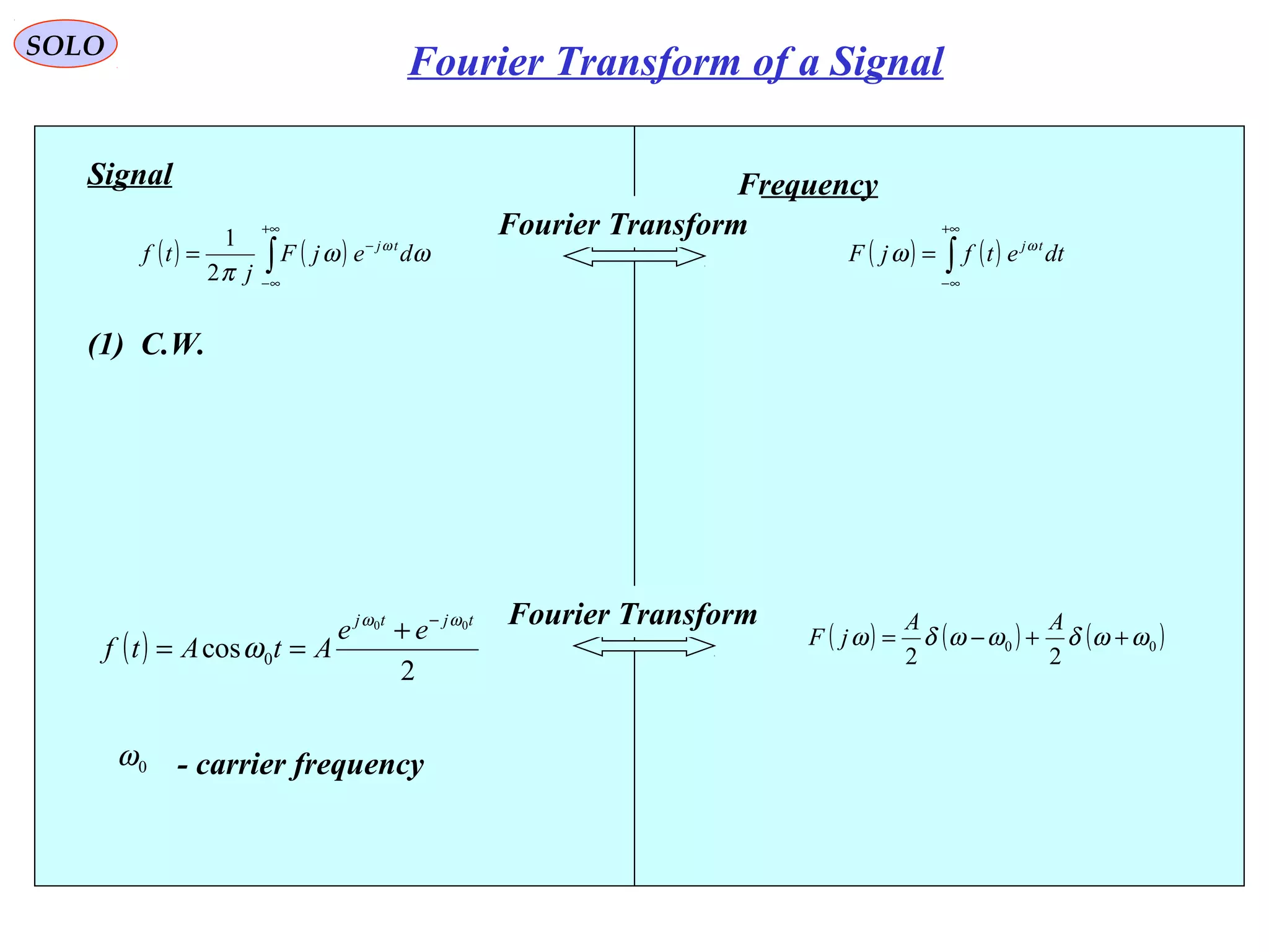
![Unmodulated
Pulse
SOLO
Energy ( ) ( ) ( )∫∫∫
+∞
∞−
+∞
∞−
+∞
∞−
=== ωω
π
dSdttsdttsEs
222
2
1
:
( )
( )
≤≤+
=
elsewhere
ttA
ts
0
0cos
: 0 τϕω
( ) ( )
( )[ ] ( ) ( )
−+
+=++=
+==
∫
∫∫
+∞
∞−
τ
ϕϕτωτ
ϕω
ϕω
τ
τ
000
2
0
00
2
0
2
00
2
2cos22cos
1
2
22cos1
2
cos
A
dtt
A
dttAdttsEs
Unmodulated Pulse](https://image.slidesharecdn.com/5-pulsecompressionwaveform-150120072751-conversion-gate02/75/5-pulse-compression-waveform-6-2048.jpg)
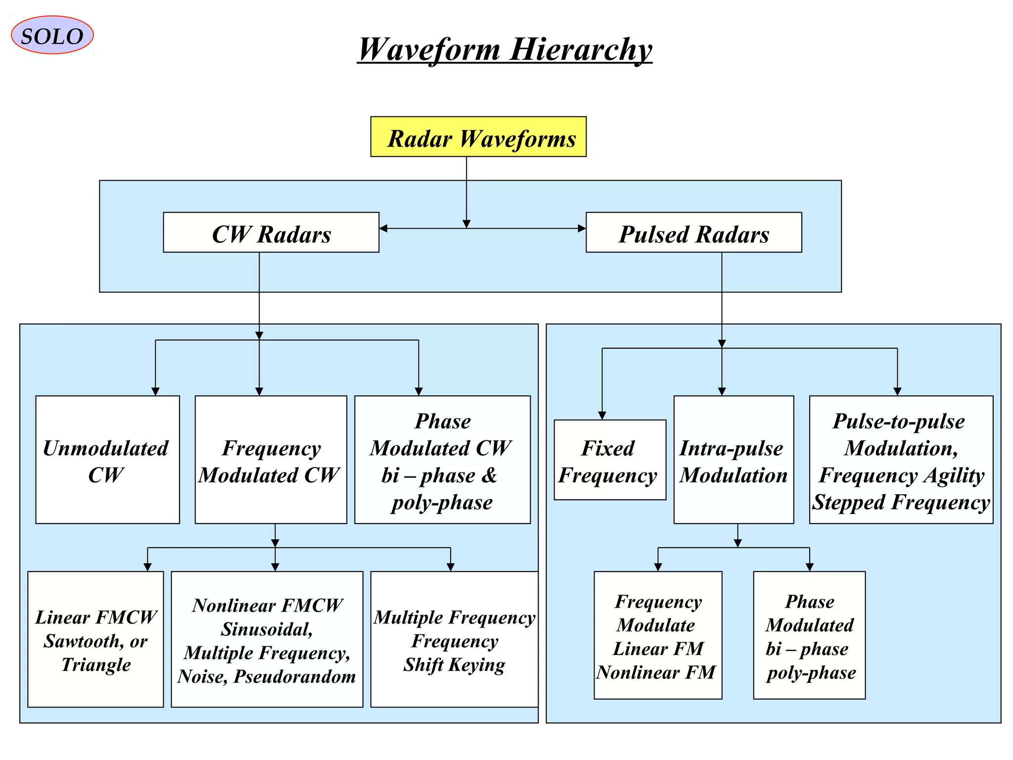
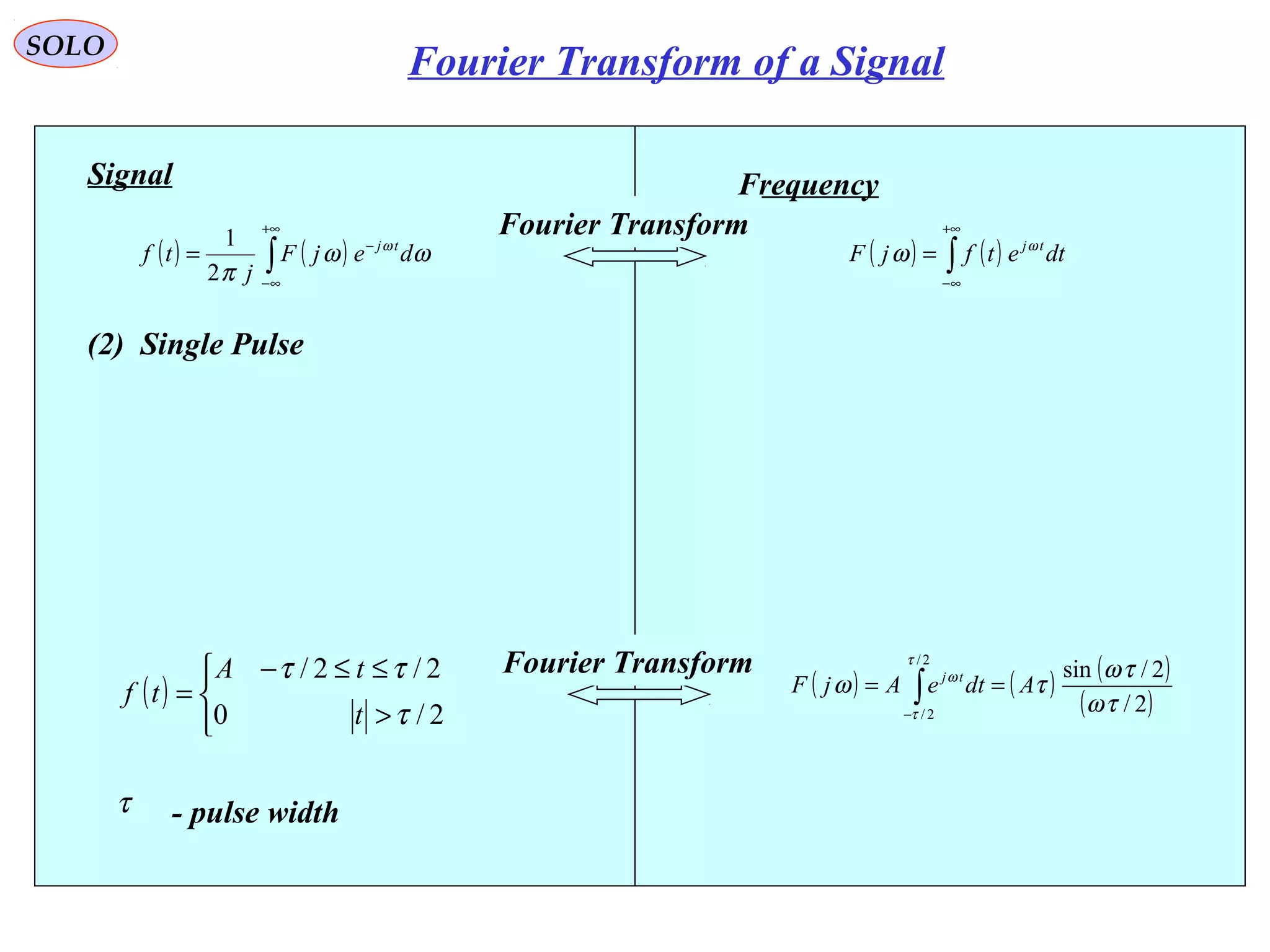
![SOLO
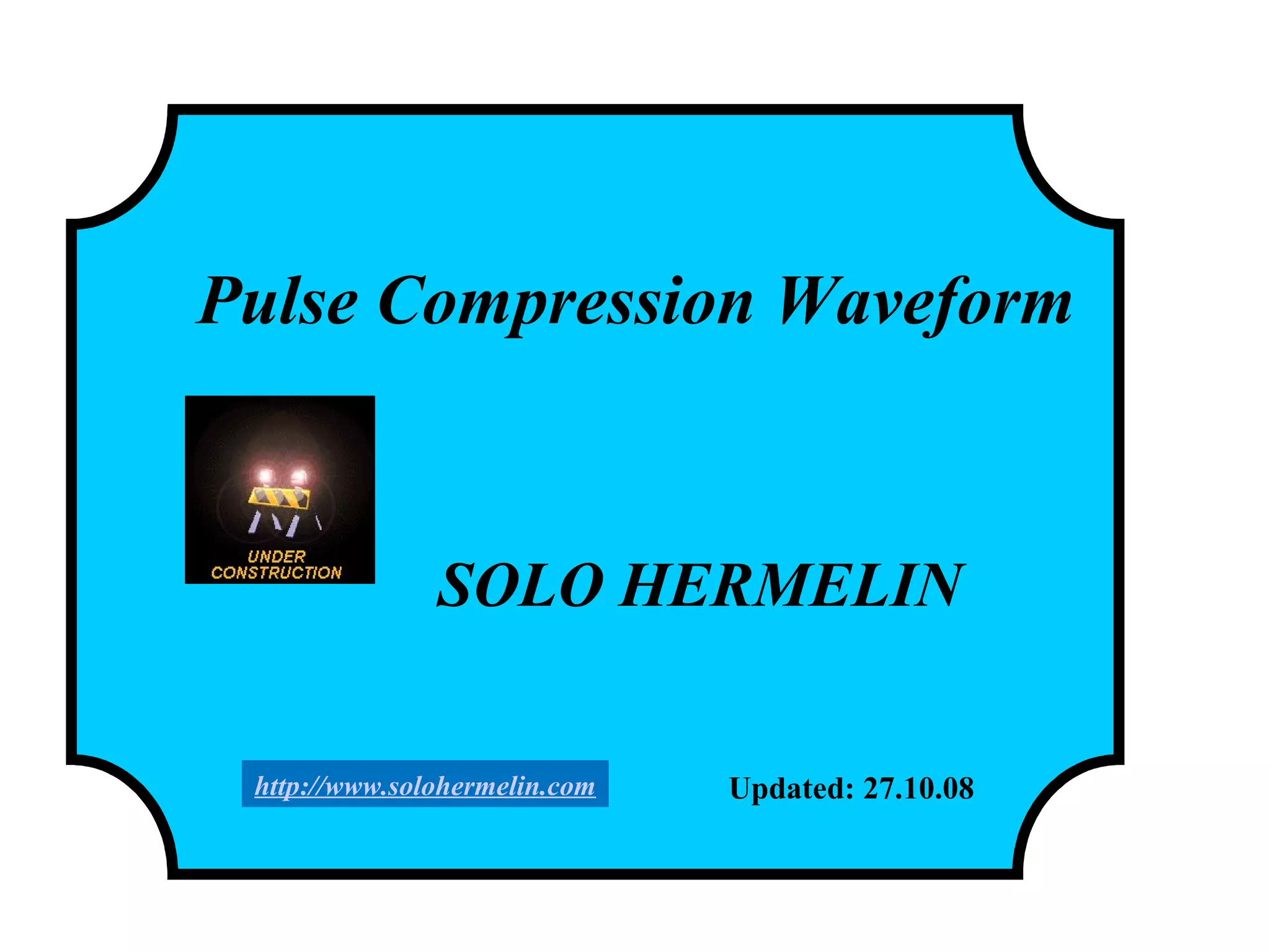
Waveform Hierarchy
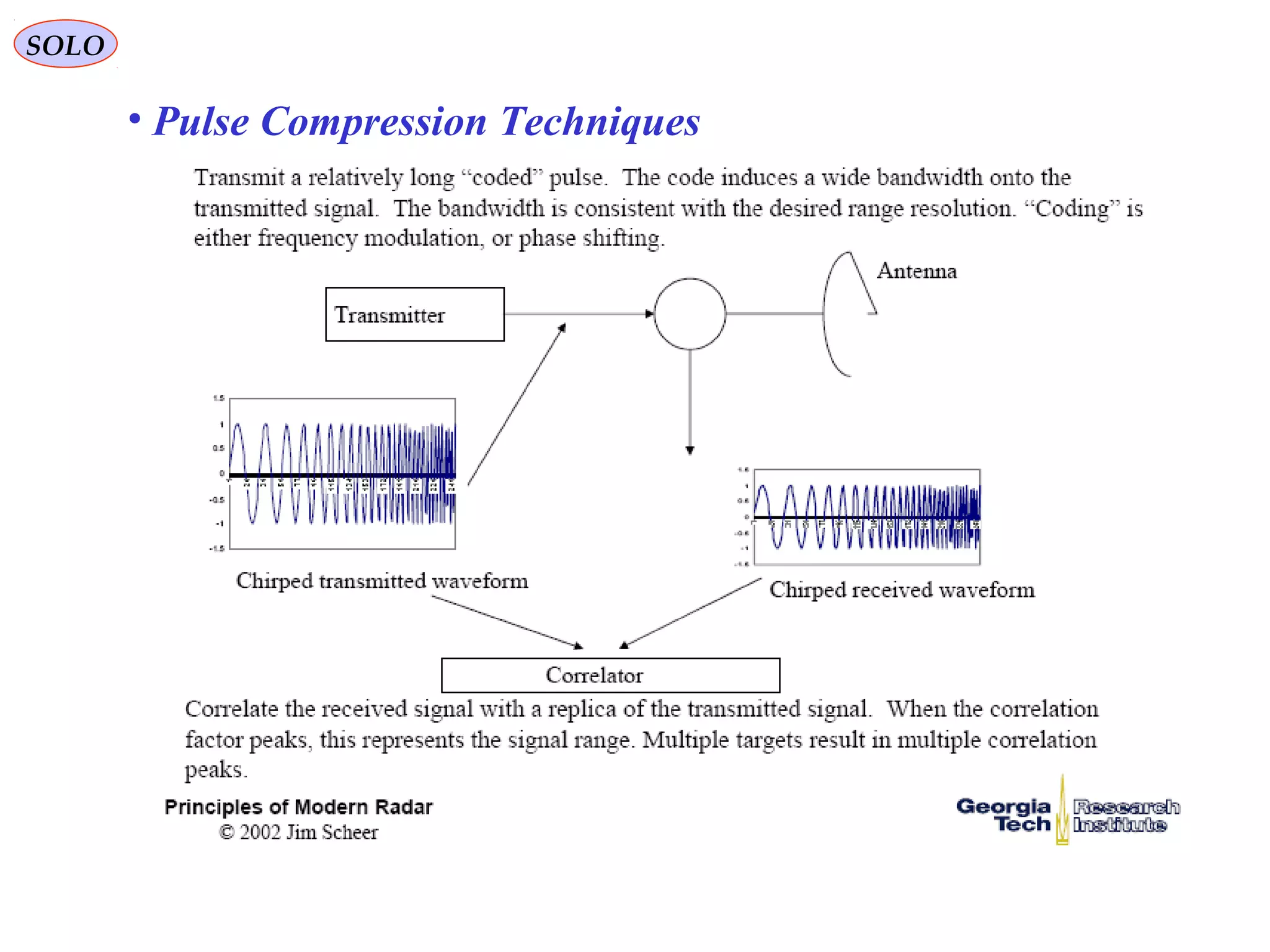
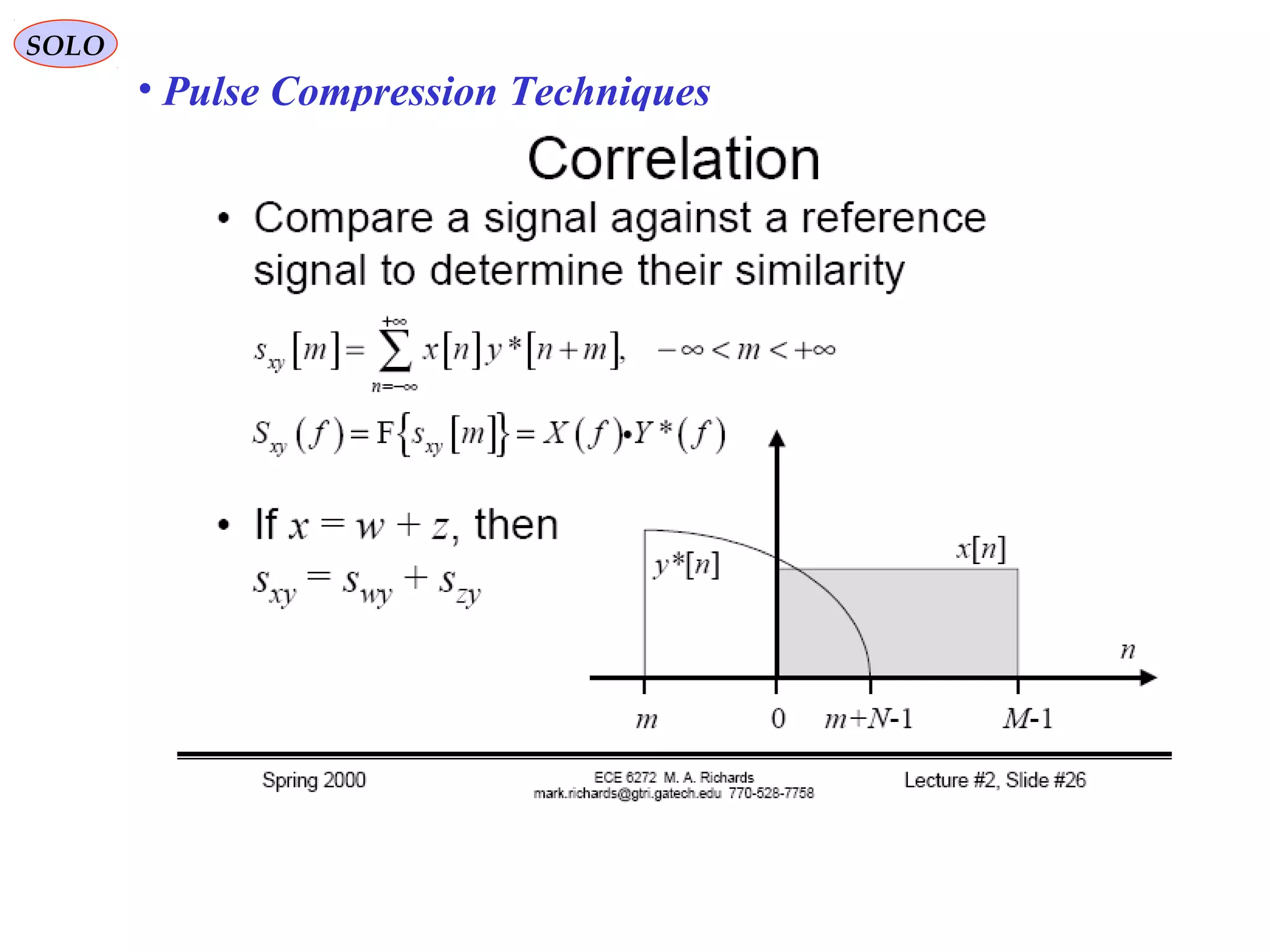
• Pulse Compression Techniques
• Wave Coding
• Frequency Modulation (FM)
- Linear
• Phase Modulation (PM)]
- Non-linear
- Pseudo-Random Noise (PRN)
- Bi-phase (0º/180º)
- Quad-phase (0º/90º/180º/270º)
• Implementation
• Hardware
- Surface Acoustic Wave (SAW) expander/compressor
• Digital Control
- Direct Digital Synthesizer (DDS)
- Software compression “filter”
Return to Table of Content](https://image.slidesharecdn.com/5-pulsecompressionwaveform-150120072751-conversion-gate02/75/5-pulse-compression-waveform-10-2048.jpg)

![SOLO
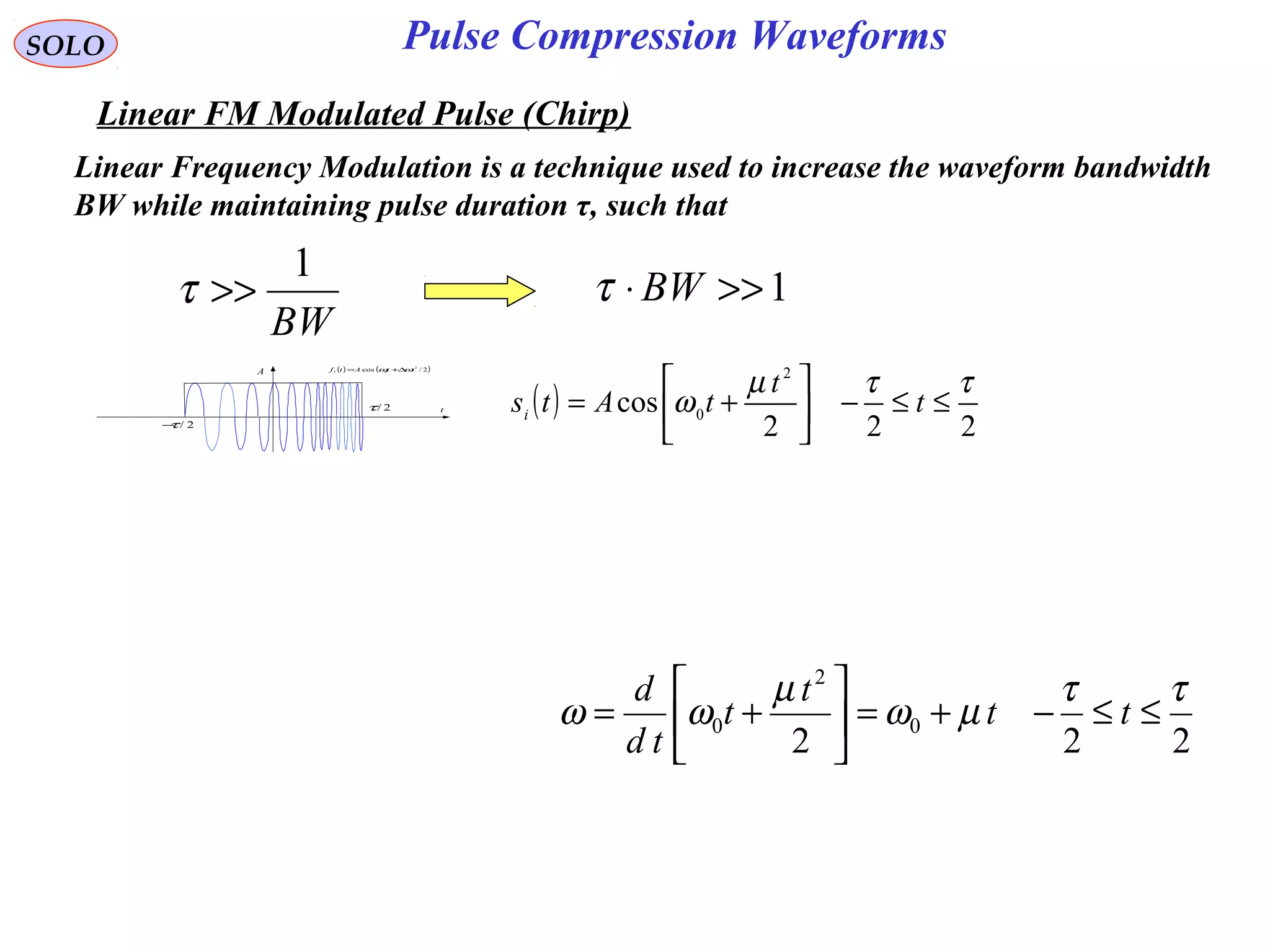
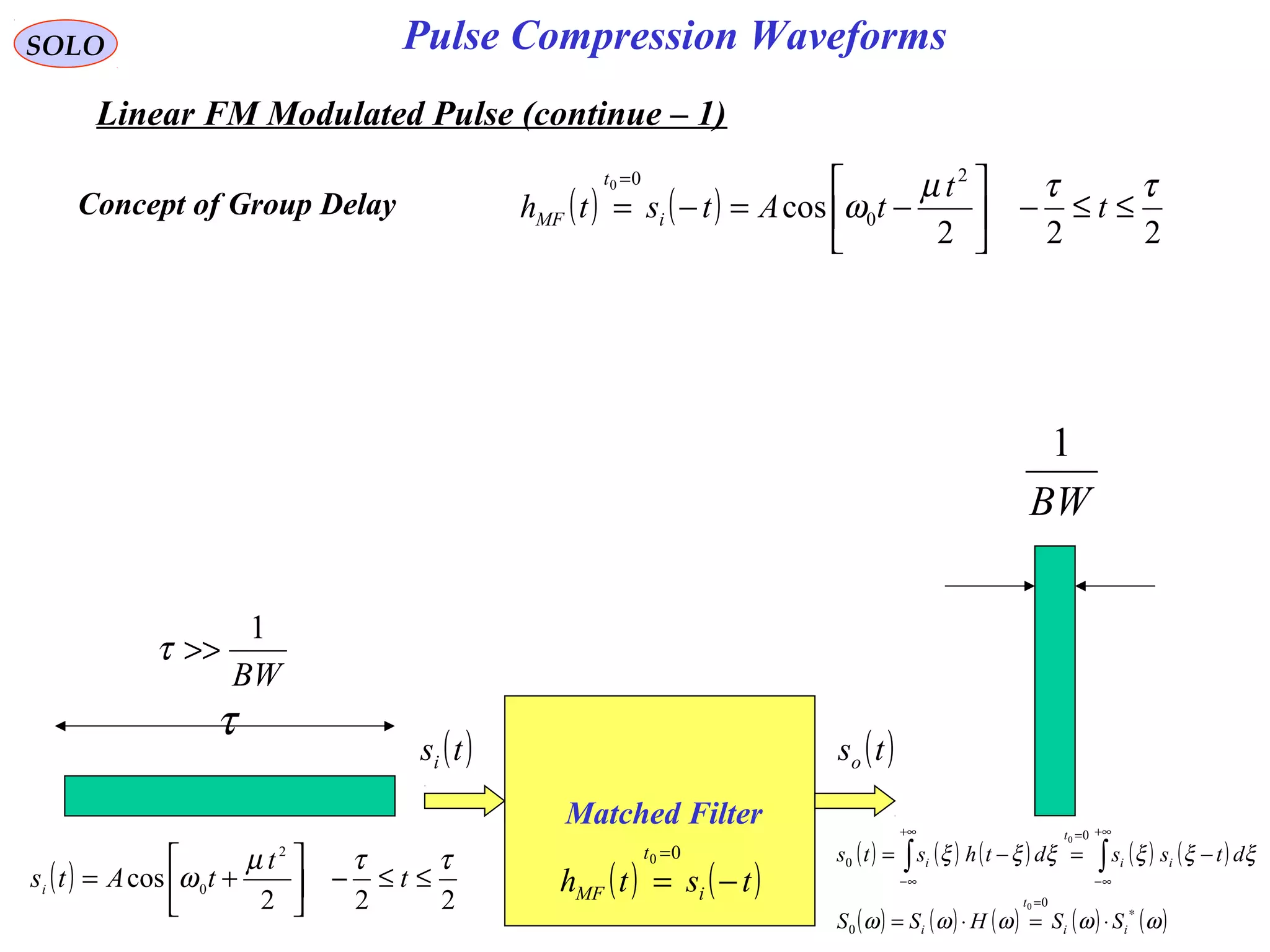
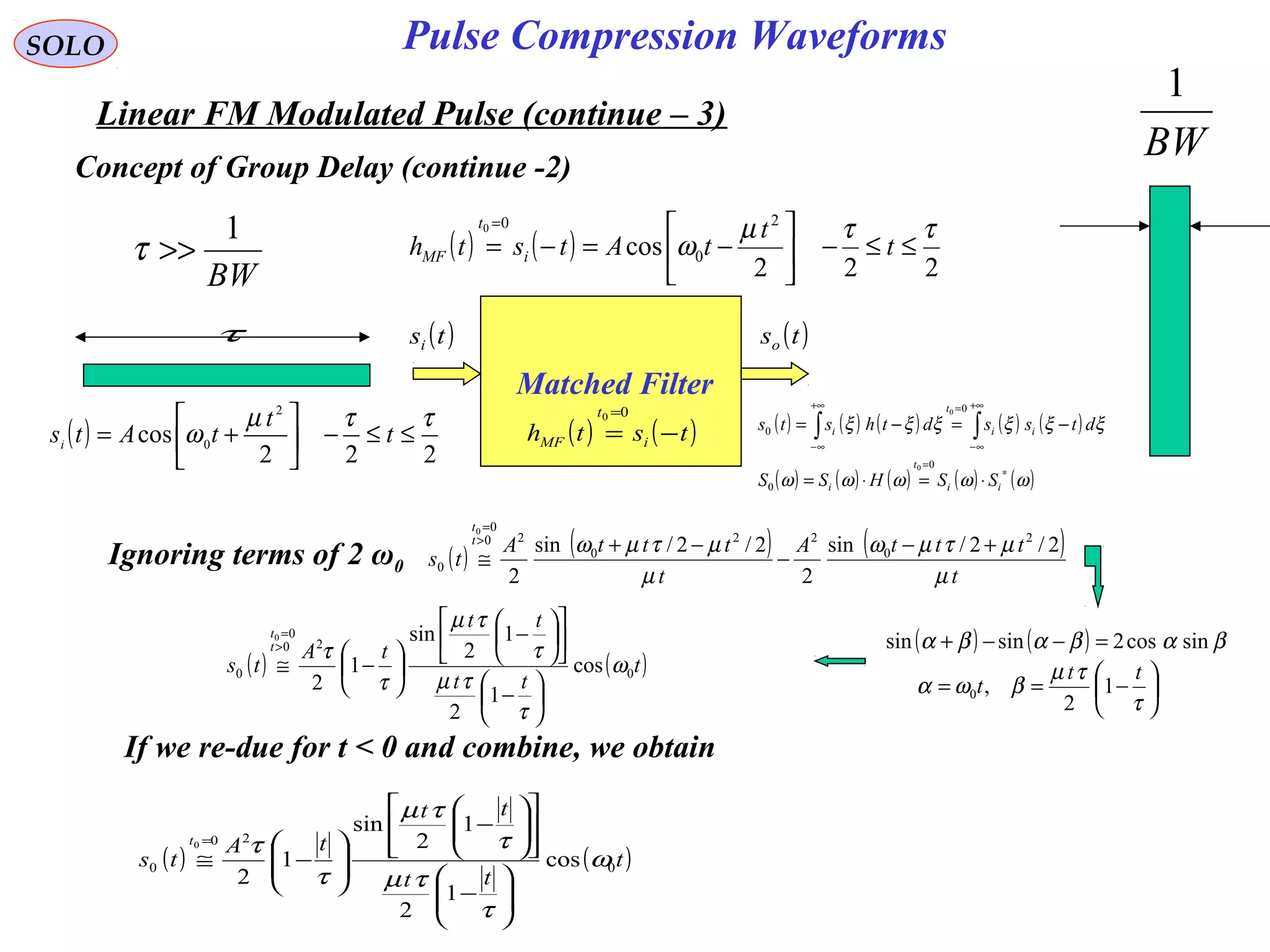
Linear FM Modulated Pulse (continue – 2)
Pulse Compression Waveforms
Concept of Group Delay (continue -1)
BW
1
>>τ
τ
BW
1
( )
222
cos
2
0
ττµ
ω ≤≤−
+= t
t
tAtsi
Matched Filter
( )tsi ( )tso
( ) ( )tsth i
t
MF −=
=00
( ) ( ) ( ) ( ) ( )
( ) ( ) ( ) ( ) ( )ωωωωω
ξξξξξξ
∗
=
+∞
∞−
=+∞
∞−
⋅=⋅=
−=−= ∫∫
ii
t
i
ii
t
i
SSHSS
dtssdthsts
0
0
0
0
0
0
( ) ( ) ( ) ( )
>≤≤+−
<+≤≤−
−
+−
+=−
0
22
0
22
2
cos
2
cos
2
0
2
0
2
tt
tt
t
tAtss ii
τ
ξ
τ
τ
ξ
τ
ξµ
ξω
ξµ
ξωξξ
( ) ( ) ( ) ( ) ( )
∫∫
+
+−
>∞+
∞−
>
=
−
+−
+=−=
2/
2/
2
0
2
0
2
00
0
0
2
cos
2
cos
0
τ
τ
ξ
ξµ
ξω
ξµ
ξωξξξ
t
t
ii
t
t
d
t
tAdtssts
( ) ( )
222
cos
2
0
00 ττµ
ω ≤≤−
−=−=
=
t
t
tAtsth i
t
MF
Ignoring terms of 2 ω0
( ) ( ) ( )
( ) ( )
t
tttA
t
tttA
t
tttA
dttt
A
ts
tt
t
t
µ
µτµω
µ
µτµω
µ
µξµω
ξµξµω
τ
τ
τ
τ
2/2/sin
2
2/2/sin
2
2/sin
2
2/cos
2
2
0
22
0
2
2/
2/
2
0
22/
2/
2
0
20
0
0
0
+−
−
−+
=
−+
=−+≅
+
+−
+
+−
>
=
∫
( ) ( ) βαβαβα coscos2coscos =−++( )[ ] ( )∫∫
+
+−
+
+−
−+++−+−=
2/
2/
2
0
22/
2/
22
0
2
2/cos
2
2/2/2cos
2
τ
τ
τ
τ
ξµξµωξµξµξµξω
tt
dtt
A
dtt
A](https://image.slidesharecdn.com/5-pulsecompressionwaveform-150120072751-conversion-gate02/75/5-pulse-compression-waveform-18-2048.jpg)
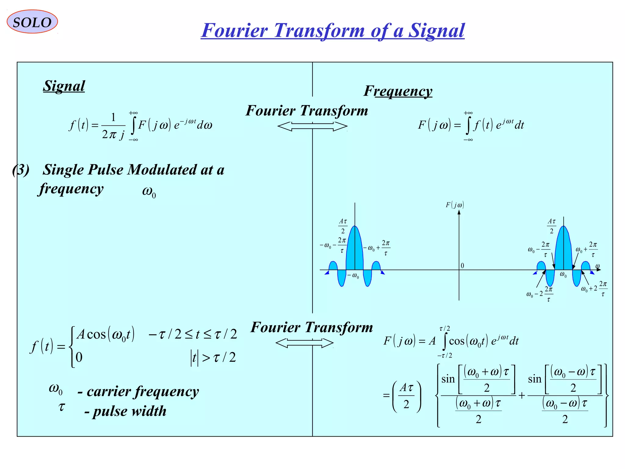
![SOLO
( ) ( )2/cos 2
03 ttAtf ωω ∆+=
t
A
2/τ−
2/τ
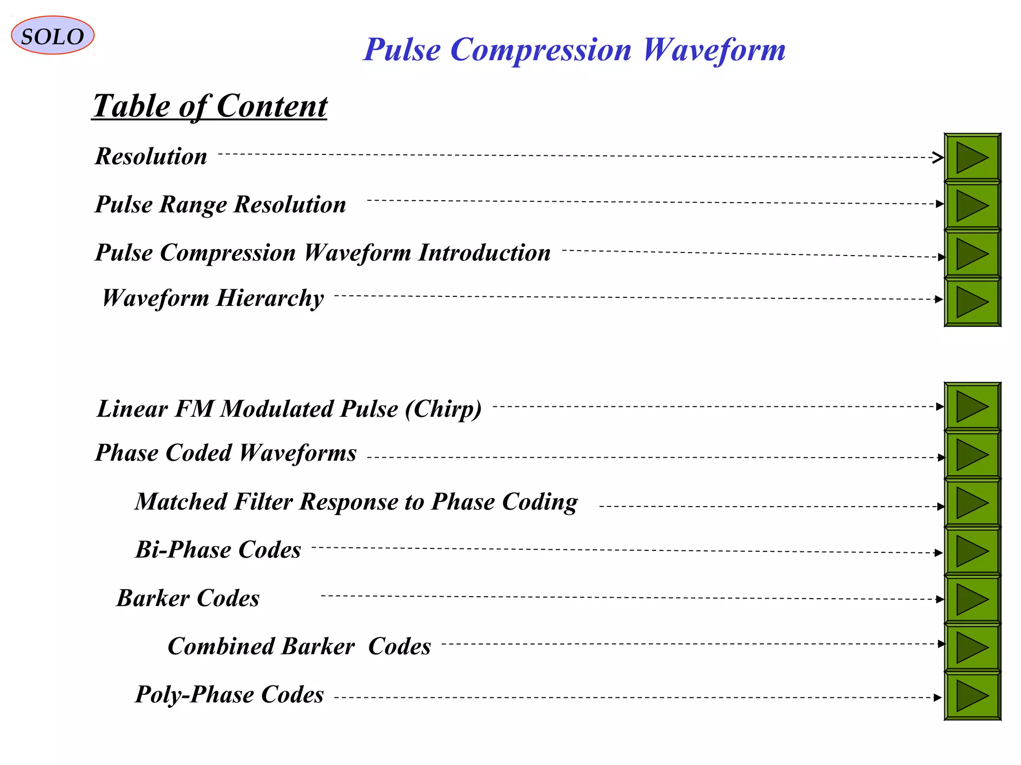
Linear FM Modulated Pulse (continue – 4)
( )
222
cos
2
0
ττµ
ω ≤≤−
+= t
t
tAtsi
The Fourier Transform is:
( ) [ ]
( ) ( )∫∫
∫
−−
−
++−+
+−=
−
+=
2/
2/
2
0
2/
2/
2
0
2/
2/
2
0
2
exp
2
1
2
exp
2
1
exp
2
cos
τ
τ
τ
τ
τ
τ
µ
ωω
µ
ωω
ω
µ
ωω
dt
t
tjAdt
t
tjA
dttj
t
tASi
∫∫ −−
+
+−
+
+
−
−
−
−=
2/
2/
2
0
2
0
2/
2/
2
0
2
0
2
exp
2
exp
22
exp
2
exp
2
τ
τ
τ
τ
µ
ωωµ
µ
ωω
µ
ωωµ
µ
ωω
dttjj
A
dttjj
A
Change variables: xt =
−
−
µ
ωω
π
µ 0
yt =
+
+
µ
ωω
π
µ 0
( ) ∫∫ −−
−
+
+
−
−=
2
1
2
1
2
exp
2
exp
22
exp
2
exp
2
2
2
0
2
2
0
Y
Y
X
X
i dt
y
jj
A
dt
x
jj
A
S
π
µ
ωωπ
µ
ωω
ω
−
−=
−
+=
µ
ωωτ
π
µ
µ
ωωτ
π
µ 0
2
0
1
2
&
2
XX
+
−=
+
+=
µ
ωωτ
π
µ
µ
ωωτ
π
µ 0
2
0
1
2
&
2
YY
Define: ( )f
n
f ∆=−=∆ πωωτµ
π
2
2
&
2
1
: 0
Pulse Compression Waveforms](https://image.slidesharecdn.com/5-pulsecompressionwaveform-150120072751-conversion-gate02/75/5-pulse-compression-waveform-20-2048.jpg)
![SOLO
( ) ( )2/cos 2
03 ttAtf ωω ∆+=
t
A
2/τ−
2/τ
Linear FM Modulated Pulse (continue – 5)
( )
222
cos
2
0
ττµ
ω ≤≤−
+= t
t
tAtsi
The Fourier Transform is:
( ) ( ) ( )
∫∫ −−
−
+
+
−
−=
2
1
2
1
2
exp
2
exp
22
exp
2
exp
2
22
0
22
0
Y
Y
X
X
i dt
y
jj
A
dt
x
jj
A
S
π
µ
ωωπ
µ
ωω
ω
The first part gives the spectrum around ω = ω0, and the second part around ω = -ω0 :
where: are Fresnel Integrals,
which have the properties:
( ) ( ) ∫∫ ==
UU
dz
z
USdz
z
UC
0
2
0
2
2
sin&
2
cos
ππ
( ) ( ) ( ) ( )USUSUCUC −=−−=− &
( ) ( ) ( ) ( ) ( ) ( )[ ]
( ) ( ) ( ) ( ) ( )[ ] ( ) ( )−+
++−=−+−
−
+
+++
−
−=
ωωωω
µ
ωω
µ
π
µ
ωω
µ
π
ω
002211
2
0
2211
2
0
2
exp
2
2
exp
2
ii
i
SSYSjYCYSjYCj
A
XSjXCXSjXCj
A
S
ωωωπωτµ
π
∆=−∆=∆=∆
2
:&2:
2
1
: 0
n
ff
Pulse Compression Waveforms](https://image.slidesharecdn.com/5-pulsecompressionwaveform-150120072751-conversion-gate02/75/5-pulse-compression-waveform-21-2048.jpg)
![SOLO
( ) ( )2/cos 2
03 ttAtf ωω ∆+=
t
A
2/τ−
2/τ
Linear FM Modulated Pulse (continue – 6)
( )
222
cos
2
0
ττµ
ω ≤≤−
+= t
t
tAtsi
The Fourier
Transform is:
ωωωπωτµ
π
∆=−∆=∆=∆
2
:&2:
2
1
: 0
n
ff
Define:
( ) ( ) ( )[ ] ( ) ( )[ ]{ }2
21
2
210
2
XSXSXCXC
A
Si
+++=− +
µ
π
ωωAmplitude Term:
Square Law Phase Term: ( ) ( )
µ
ωω
ω
2
2
0
1
−
−=Φ
Residual Phase Term: ( ) ( ) ( )
( ) ( ) 4
1tan
5.05.0
5.05.0
tantan 11
1
21
211
2
π
ω
τ
==
+
+
→
+
+
=Φ −−
>>∆
−
f
XCXC
XSXS
( ) ( )nfXnfX −∆=+∆= 1
2
&1
2
21
ττ
( ) ( ) ( ) ( ) ( ) ( )[ ]
( ) ( ) ( ) ( ) ( )[ ] ( ) ( )−+
++−=−+−
−
+
+++
−
−=
ωωωω
µ
ωω
µ
π
µ
ωω
µ
π
ω
002211
2
0
2211
2
0
2
exp
2
2
exp
2
ii
i
SSYSjYCYSjYCj
A
XSjXCXSjXCj
A
S
( )ω2Φ( ) +
− ωω0iS
Pulse Compression Waveforms](https://image.slidesharecdn.com/5-pulsecompressionwaveform-150120072751-conversion-gate02/75/5-pulse-compression-waveform-23-2048.jpg)
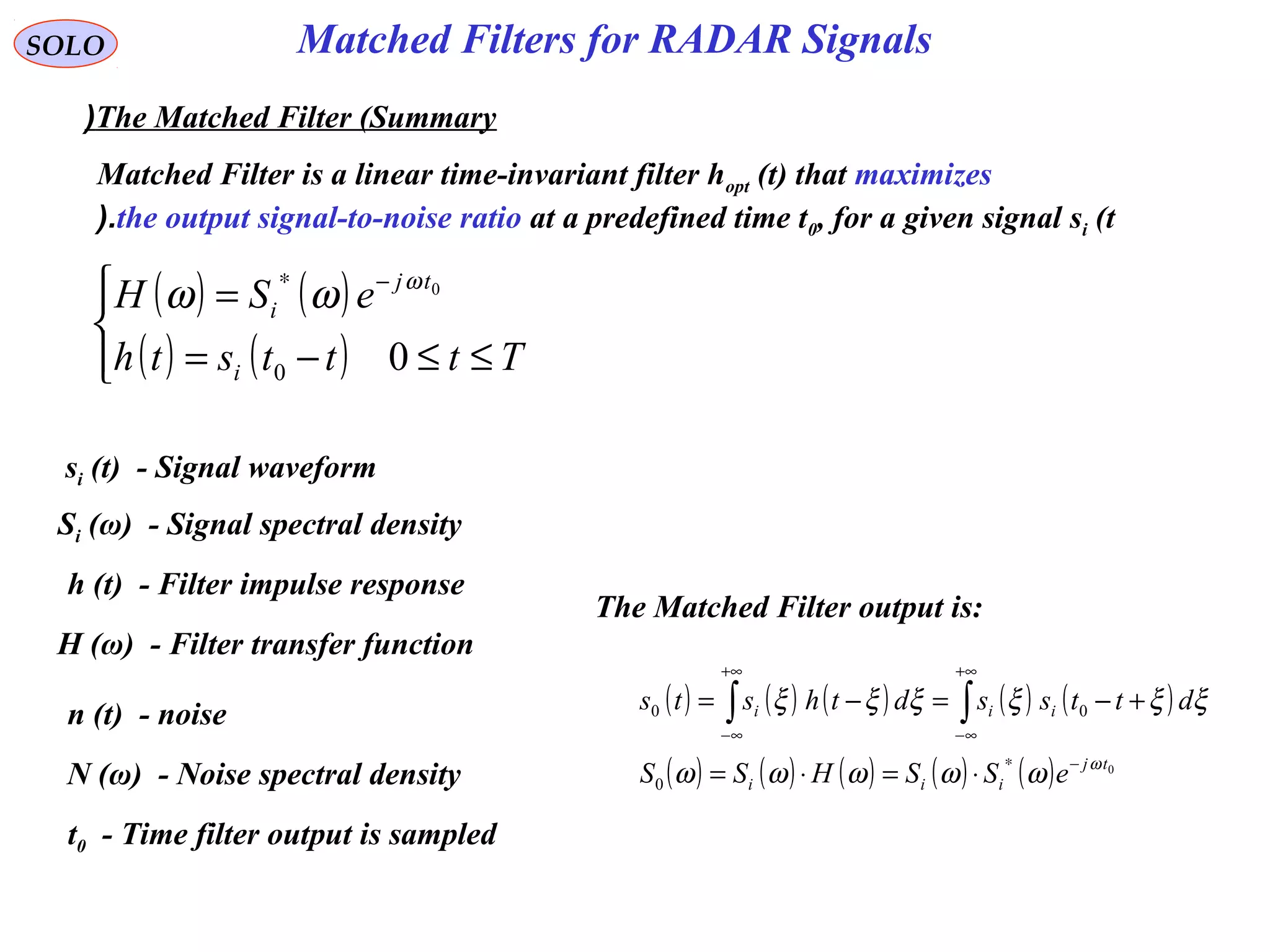
![Matched Filters for RADAR SignalsSOLO
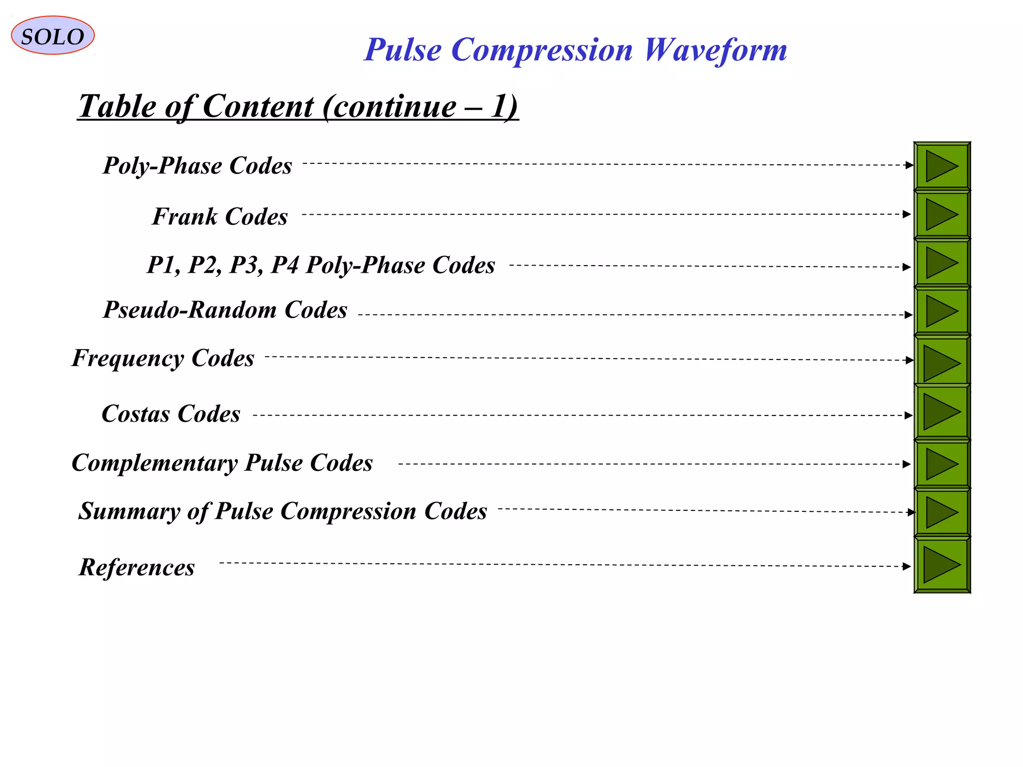
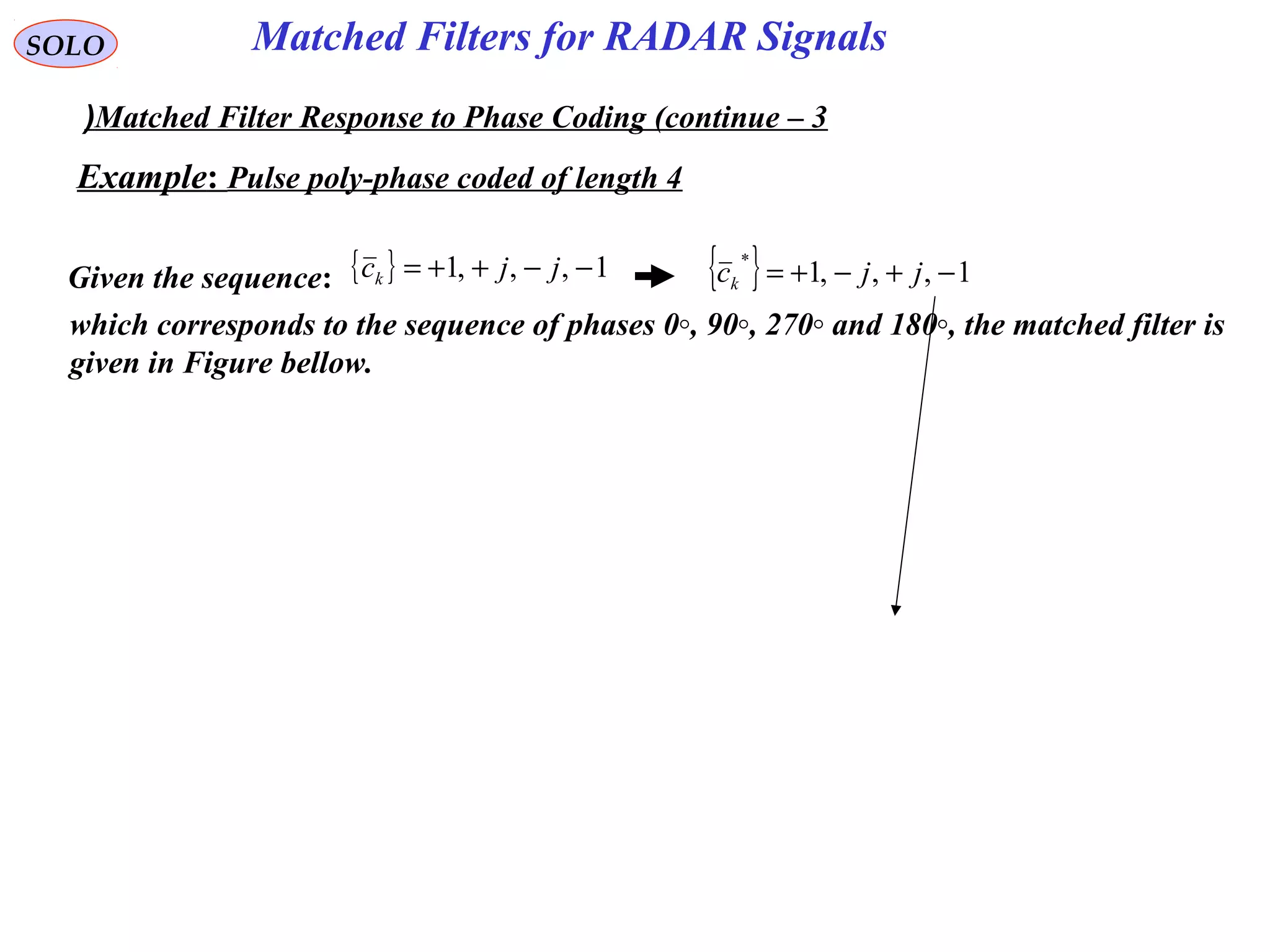
Matched Filter Response to Phase Coding
( ) ( ) ( ) ( ) ( )tjtgtjtgts 00 exp
2
1
exp
2
1
ωω −+= ∗
( ) ( ) ( )
∆<<
=∆−= ∑
−
= elsewhere
tt
tftptfctg
M
p
p
0
011
0
Let the signal be a phase-modulated carrier, in which the modulation is in discrete and
equal steps Δt. The complex envelope of the signal can be described by a sequence of
complex numbers , such thatkc
( ) [ ] ( ) ( )∫
+∞
∞−
∗
+−−= dtttgtgtjgo 000exp
2
1
τωτ
Constant Phase
Matched Filter output envelope (change t ↔τ):
( )ttk ∆<≤+∆→ τττ 0
tMt ∆=0
( ) [ ] ( ) ( )[ ]
[ ] ( )[ ]
( )
∑ ∫
∫∑
−
=
∆+
∆
∗
+∞
∞−
∗
−
=
∆−+−∆−=
∆−+−∆−∆−=+∆
1
0
1
0
1
0
0
exp
2
1
exp
2
1
M
p
tp
tp
p
M
p
po
dttkMtgctMj
dttkMtgtptfctMjtkg
τω
τωτ
Change variable of integration to t1 = t – τ + (M - k) Δt
( ) [ ] ( )
( )
( )
∑ ∫
−
=
−∆+−+
−∆−+
∗
∆−=+∆
1
0
1
110exp
2
1 M
p
tkMp
tkMp
po dttgctMjtkg
τ
τ
ωτ](https://image.slidesharecdn.com/5-pulsecompressionwaveform-150120072751-conversion-gate02/75/5-pulse-compression-waveform-27-2048.jpg)
![Matched Filters for RADAR SignalsSOLO
Matched Filter Response to Phase Coding (continue – 1(
Matched Filter output envelope for a Phase Coding is:
( ) [ ] ( )[ ]
( )
∑ ∫
−
=
∆+
∆
∗
∆−+−∆−=+∆
1
0
1
0exp
2
1 M
p
tp
tp
po dttkMtgctMjtkg τωτ
Change variable of integration to t1 = t – τ + (M - k) Δt
( ) [ ] ( )
( )
( )
[ ] ( )
( )
( )
( )
( )
( )
∑ ∫∫∑ ∫
−
=
−∆+−+
∆−+
∗
∆−+
−∆−+
∗
−
=
−∆+−+
−∆−+
∗
+∆−=∆−=+∆
1
0
1
11110
1
0
1
110 exp
2
1
exp
2
1 M
p
tkMp
tkMp
tkMp
tkMp
p
M
p
tkMp
tkMp
po dttgdttgctMjdttgctMjtkg
τ
τ
τ
τ
ωωτ
( ) ( ) ( )
( ) ( ) ( ) τ
τ
−∆+−+<<∆−+=
∆−+<<−∆−+=
−+
∗
−−+
∗
tkMpttkMpctg
tkMpttkMpctg
kMp
kMp
11
*
1
11
*
1
( ) [ ] ∑ ∫∫
−
=
−∆
−+
−
−−+
+∆−=+∆
1
0 0
1
*
0
11
*
0exp
2
1 M
p
t
kMpkMppo dtcdtcctMjtkg
τ
τ
ωτ
( ) [ ] ∑
−
=
−+−−+
∆
−+
∆
∆−
∆
=+∆
1
0
*
1
*
0 1exp
2
1 M
p
kMpkMppo
t
c
t
cctMj
t
tkg
ττ
ωτ
This equation describes straight lines in the complex plane, that can have corners only at
τ = 0. At those corners
( ) [ ] ∑
−
=
−+∆−
∆
=∆
1
0
*
0exp
2
1 M
p
kMppo cctMj
t
tkg ω
Constant Phase](https://image.slidesharecdn.com/5-pulsecompressionwaveform-150120072751-conversion-gate02/75/5-pulse-compression-waveform-28-2048.jpg)
![Matched Filters for RADAR SignalsSOLO
Matched Filter Response to Phase Coding (continue – 2(
Matched Filter output envelope for a Phase Coding is:
( ) [ ] ∑
−
=
−+−−+
∆
−+
∆
∆−
∆
=+∆
1
0
*
1
*
0 1exp
2
1 M
p
kMpkMppo
t
c
t
cctMj
t
tkg
ττ
ωτ
This equation describes straight lines in the complex plane, that can have corners only at
τ = 0. At those corners
( ) [ ] ∑
−
=
−+∆−
∆
=∆
1
0
*
0exp
2
1 M
p
kMppo cctMj
t
tkg ω
Constant Phase
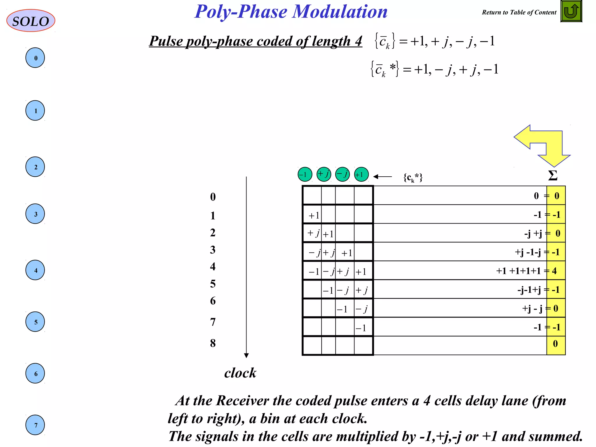
We can see that is the discrete autocorrelation function for the
observation time t0 = M Δt (the time the received Radar signal return is expected)
∑
−
=
−+
1
0
*
M
p
kMpp cc](https://image.slidesharecdn.com/5-pulsecompressionwaveform-150120072751-conversion-gate02/75/5-pulse-compression-waveform-29-2048.jpg)
![SOLO Pulse Compression Techniques
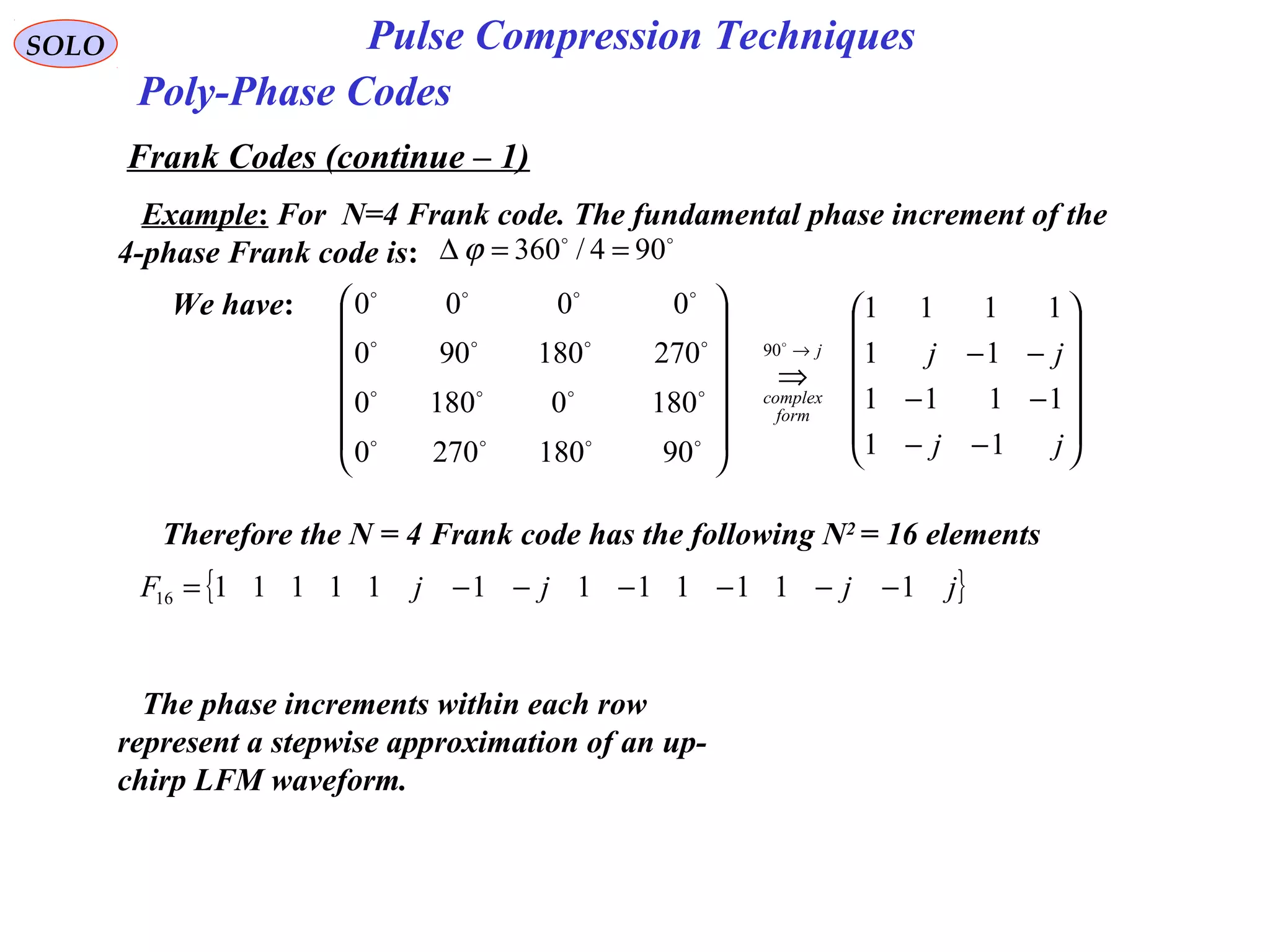
P1, P2, P3, P4 Poly-Phase Codes
The phase-code pulses envelope is given by: ( ) ( ) ( )
∑=
−−
=
N
m
m
mt
recj
NT
tg
1 '
1
exp
1
τ
ϕ
The phases φm are chosen such that the autocorrelation function has the smallest
Peak-to-sidelobe ratio (PSR), for a certain code length. PSR is bounded from bellow
by the code length N
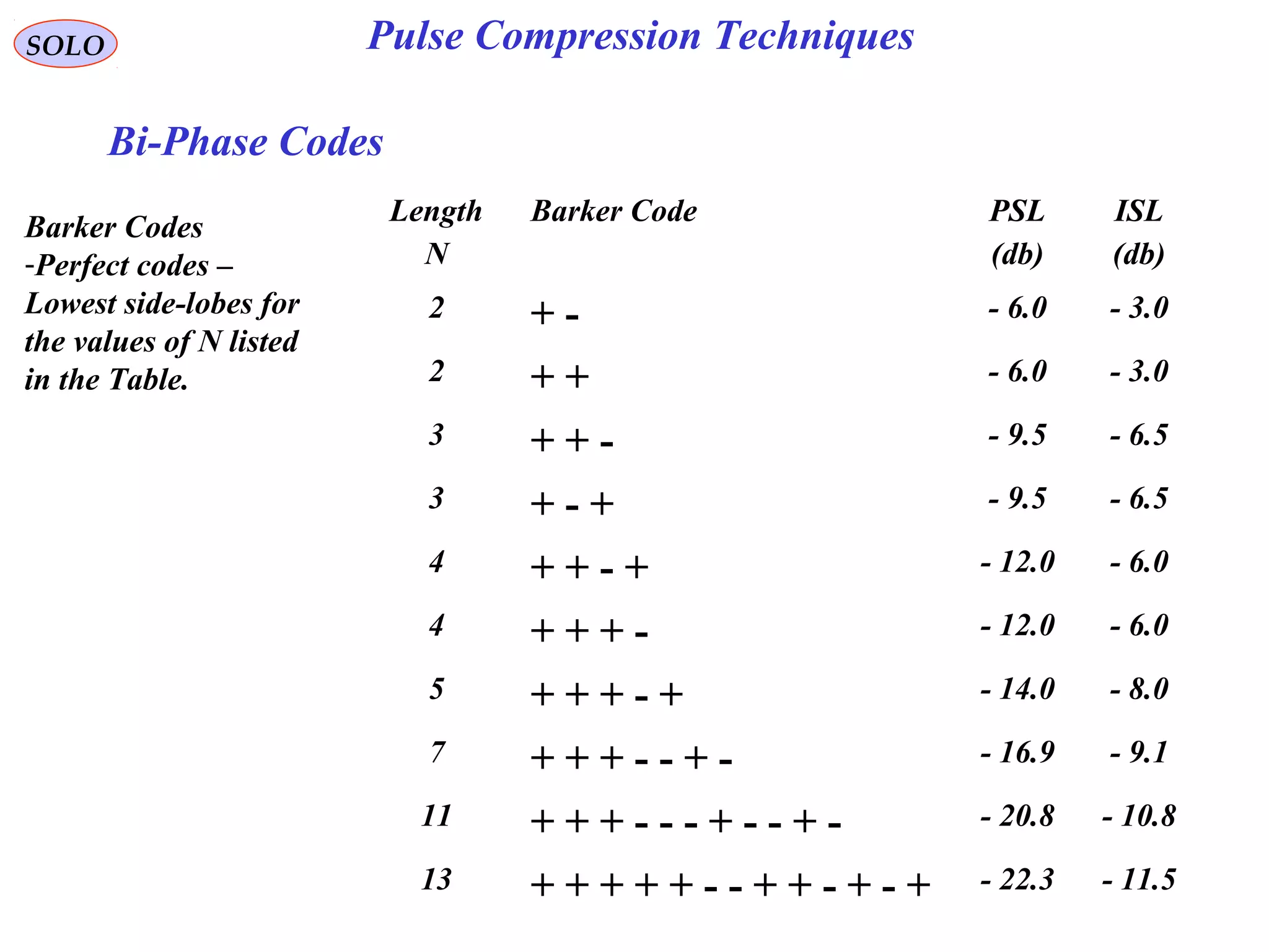
( )NPSR log20=
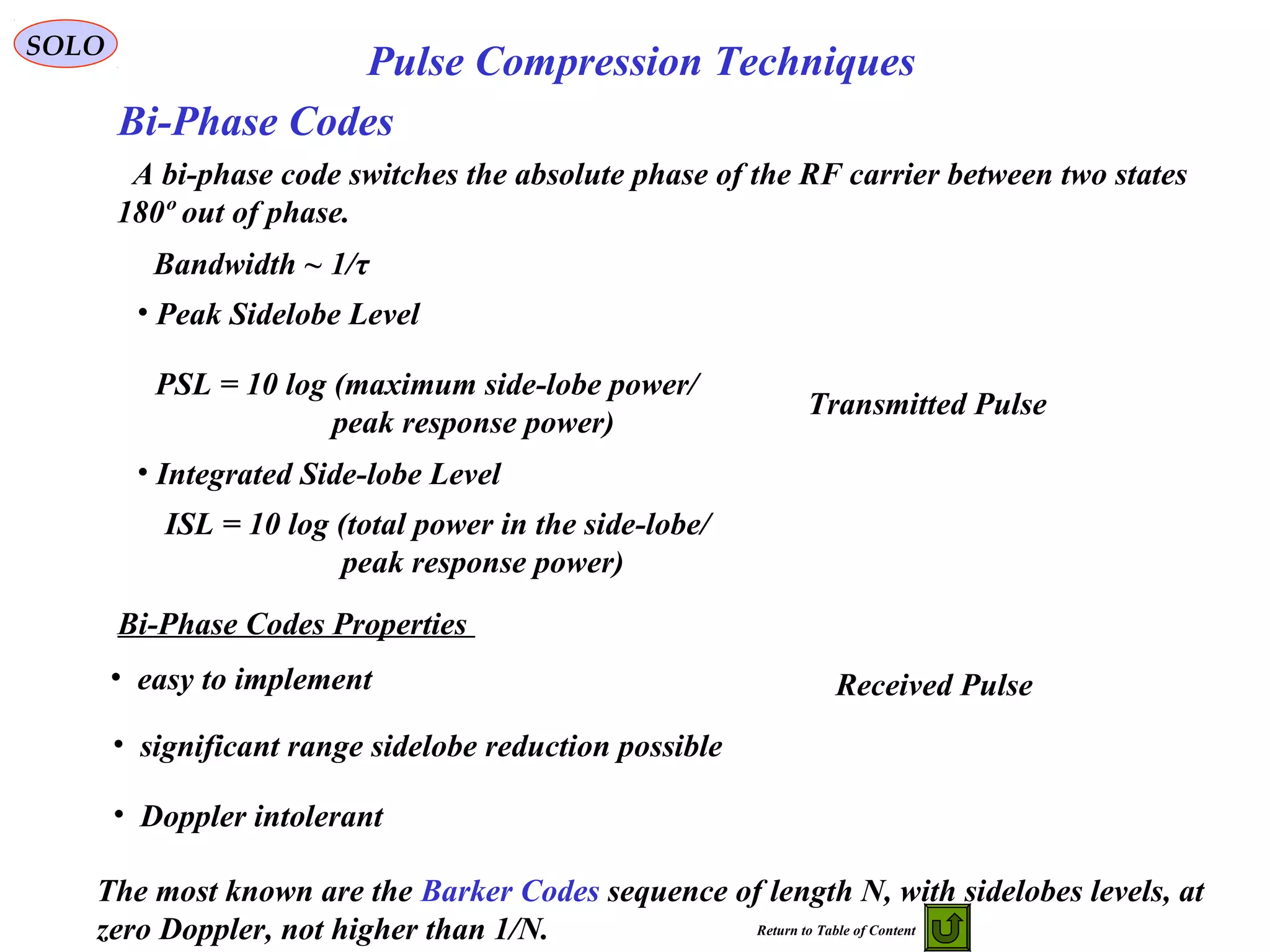
Binary phase codes use only φm=0 or π. The main drawback of binary codes, such as
Barker codes or m-sequences is their sensitivity to Doppler shift.
Poly-phase codes are not restricted on code elements and are generated from phase
history of frequency-modulated pulse. The Frank code and the P1 and P2 codes,
The modified version of Frank code, are derived from the linear stepped frequency
Modulation. These three codes are only applicable for perfect square length (N = L2
),
and can be expressed as:
( ) ( )
( ) ( )[ ] ( )[ ]
( )[ ] ( )[ ]jLiL
L
P
jLiLj
L
P
ji
L
Frank
ji
ji
ji
−+−+=
−−−+−=
−−=
2/12/1
2
:2
1211
2
:1
11
2
:
,
,
,
π
ϕ
π
ϕ
π
ϕ](https://image.slidesharecdn.com/5-pulsecompressionwaveform-150120072751-conversion-gate02/75/5-pulse-compression-waveform-47-2048.jpg)

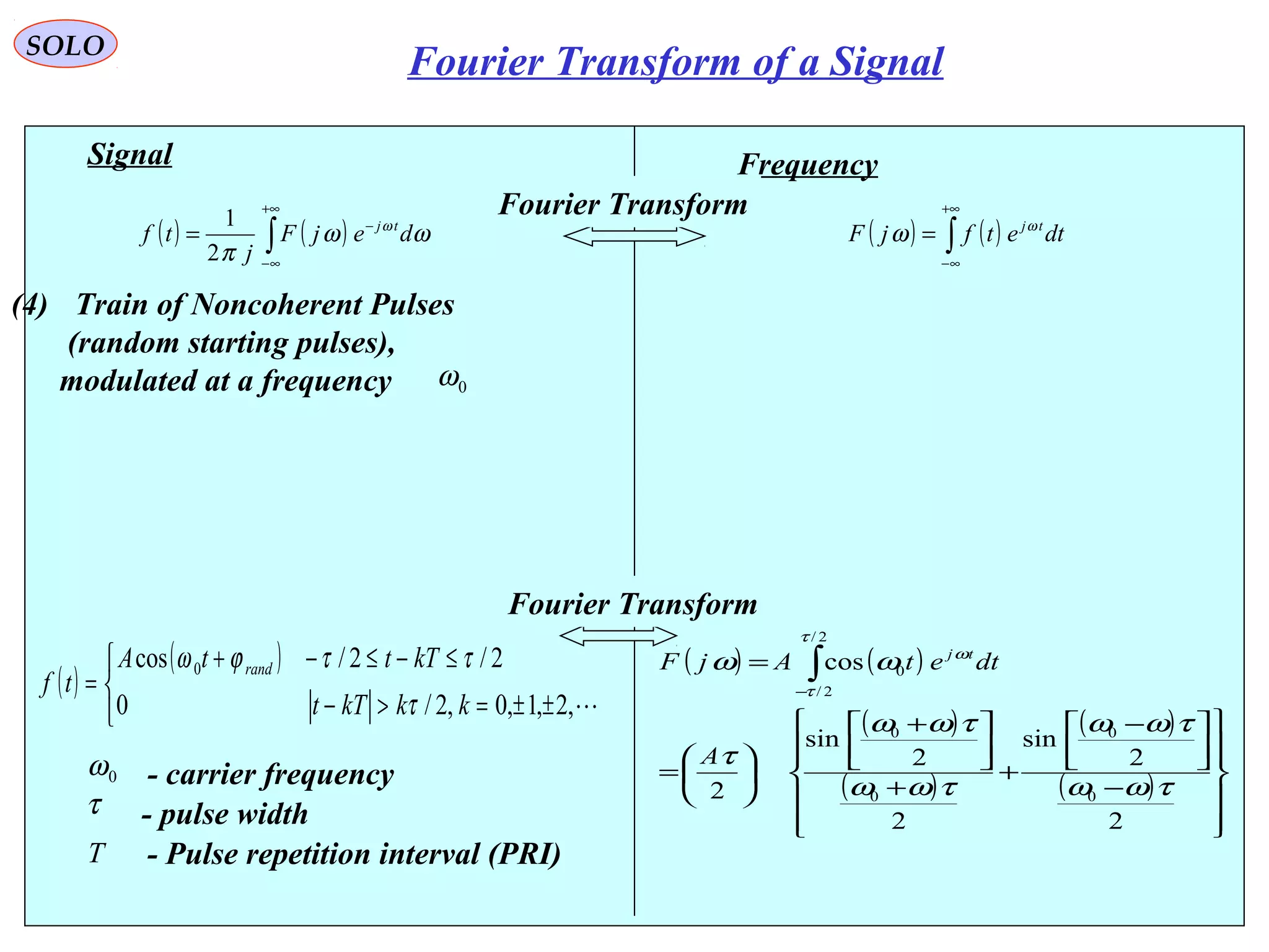
![( ) ( )∫
+∞
∞−
−
= ωω
π
ω
dejF
j
tf tj
2
1
Signal
( )
( )
( ) ( )( ) ( )( )[ ]
−++
+=
±±=>−
≤−≤−
=
∑
∞
=1
000
0
coscos
2
2
sin
cos
,2,1,0,2/0
2/2/cos
n
PRPR
PR
PR
series
Fourier
tntn
n
n
t
T
A
kkkTt
kTttA
tf
ωωωω
τω
τω
ω
τ
τ
ττω
τ - pulse width
Frequency
( ) ( )∫
+∞
∞−
= dtetfjF tjω
ω
Fourier Transform
Fourier Transform
0ω - carrier frequency
5) Train of Coherent Pulses,
of infinite length,
modulated at a frequency 0ω
T - Pulse repetition interval (PRI)
( ) ( ) ( ){
( ) ( ) ( ) ( )[ ]
+−+−+−−++
+
−+=
∑
∞
=1
0000
00
2
2
sin
2
n
PRPRPRPR
PR
PR
nnnn
n
n
T
A
jF
ωωδωωδωωδωωδ
τω
τω
ωδωδ
τ
ω
T/1 - Pulse repetition frequency (PRF)
TPR /2πω =
SOLO
Fourier Transform of a Signal](https://image.slidesharecdn.com/5-pulsecompressionwaveform-150120072751-conversion-gate02/75/5-pulse-compression-waveform-68-2048.jpg)
![( ) ( )∫
+∞
∞−
−
= ωω
π
ω
dejF
j
tf tj
2
1
Signal
( )
( )
( ) ( )( ) ( )( )[ ]
−++
+=
±±=>−
≤−≤−
=
∑
∞
=
≤≤−
1
000
22
0
coscos
2
2
sin
cos
2/,,2,1,0,2/0
2/2/cos
n
PRPR
PR
PRNT
t
NT
tntn
n
n
t
T
A
NkkkTt
kTttA
tf
ωωωω
τω
τω
ω
τ
τ
ττω
τ - pulse width
Frequency
( ) ( )∫
+∞
∞−
= dtetfjF tjω
ω
Fourier Transform
Fourier Transform
0ω - carrier frequency
6) Train of Coherent Pulses,
of finite length N T,
modulated at a frequency 0ω
T - Pulse repetition interval (PRI)
( )
( )
( )
( )
( )
( )
( )
( )
( )
( )
( )
( )
( )
−−
−−
+
+−
+−
+
+
+
+
−+
−+
+
++
++
+
+
+
=
∑
∑
∞
=
∞
=
1
0
0
0
0
0
0
1
0
0
0
0
0
0
2
2
sin
2
2
sin
2
2
sin
2
2
sin
2
2
sin
2
2
sin
2
2
sin
2
2
sin
2
n
PR
PR
PR
PR
PR
PR
n
PR
PR
PR
PR
PR
PR
TN
n
TN
n
TN
n
TN
n
n
n
TN
TN
TN
n
TN
n
TN
n
TN
n
n
n
TN
TN
T
A
jF
ωωω
ωωω
ωωω
ωωω
τω
τω
ωω
ωω
ωωω
ωωω
ωωω
ωωω
τω
τω
ωω
ωω
τ
ω
T/1 - Pulse repetition frequency (PRF)
TPR /2πω =
SOLO
Fourier Transform of a Signal](https://image.slidesharecdn.com/5-pulsecompressionwaveform-150120072751-conversion-gate02/75/5-pulse-compression-waveform-69-2048.jpg)
![Signal
( ) ( )
+=
±±=>−
≤−≤−
= ∑
∞
=1
1 cos
2
2
sin
21
,2,1,0,2/0
2/2/
n
PR
PR
PR
Series
Fourier
tn
n
n
T
A
kkkTt
kTtA
tf ω
τω
τω
τ
τ
ττ
τ - pulse width
0ω - carrier frequency
6) Train of Coherent Pulses,
of finite length N T,
modulated at a frequency 0ω
T - Pulse repetition interval (PRI)
T/1 - Pulse repetition frequency (PRF)
TPR /2πω =
( ) ( )tAtf 03 cos ω=
t
A A
( )tf1
t
2
τ
2
τ
−T
A
T T
2
2
τ+T
2
2
τ−T
T T
2
τ− 2
τ+T
( )tf2
t
TN
2/TN2/TN−
( ) ( ) ( ) ( )tftftftf 321 ⋅⋅=
( ) ( ) ( ) ( )
( )
( ) ( )( ) ( )( )[ ]
−++
+=
±±=>−
≤−≤−
=⋅⋅=
∑
∞
=
≤≤−
1
000
22
0
321
coscos
2
2
sin
cos
2/,,2,1,0,2/0
2/2/cos
n
PRPR
PR
PRNT
t
NT
tntn
n
n
t
T
A
NkkkTt
kTttA
tftftftf
ωωωω
τω
τω
ω
τ
τ
ττω
( )
>
≤≤−
=
2/0
2/2/1
2
TNt
TNtTN
tf ( ) ( )ttf 03 cos ω=
SOLO
Fourier Transform of a Signal](https://image.slidesharecdn.com/5-pulsecompressionwaveform-150120072751-conversion-gate02/75/5-pulse-compression-waveform-70-2048.jpg)

The document discusses pulse compression waveforms in radar systems, emphasizing their role in improving range resolution and waveform energy decoupling. It details various coding techniques, such as linear FM modulation and matched filtering, to enhance signal clarity and distinguishability between targets. Furthermore, it covers the mathematical foundation and implications of these waveforms in radar performance.
Introduces pulse compression waveforms and their hierarchy, including types of modulation (Chirp, Barker codes, etc.).
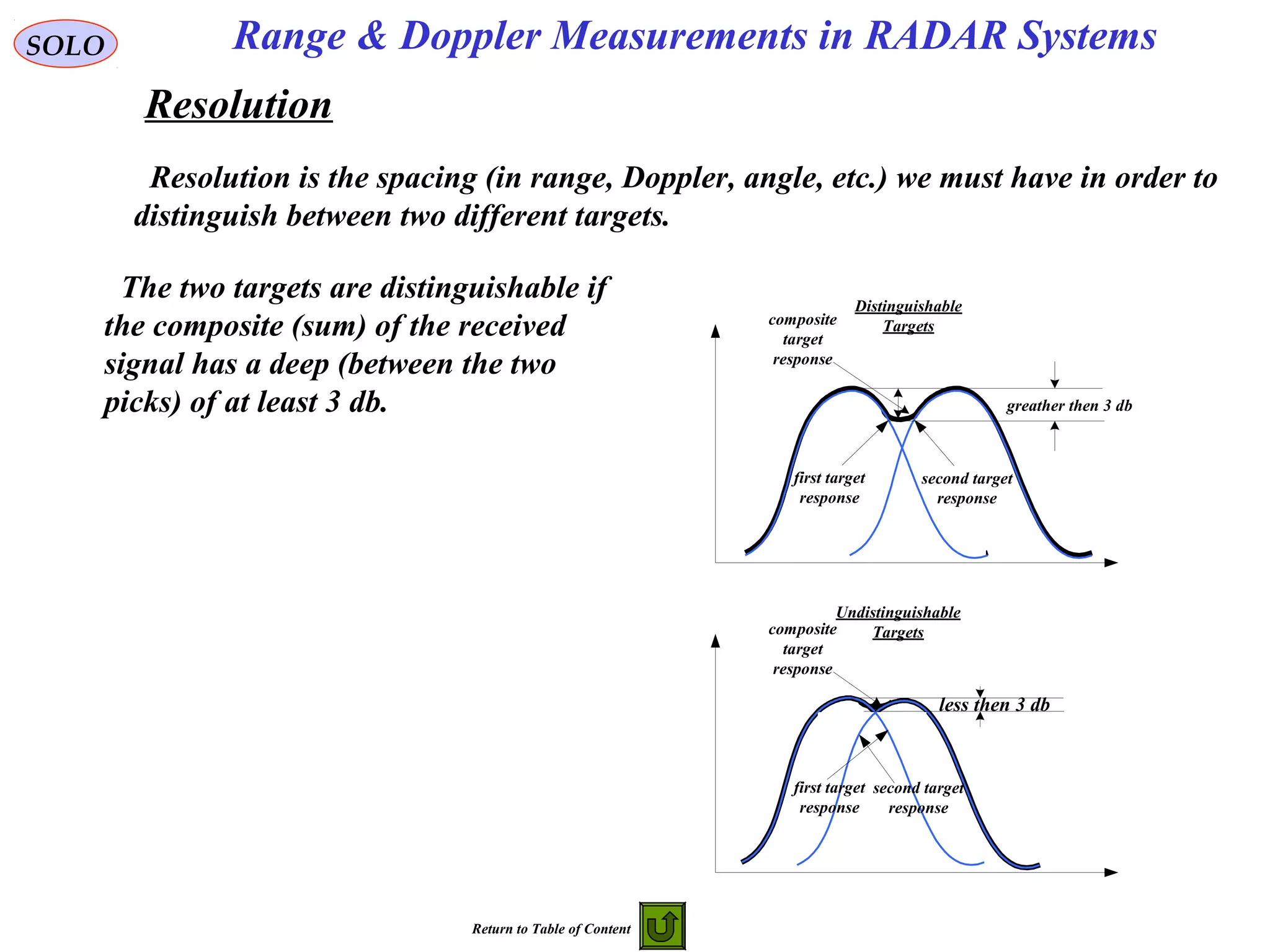
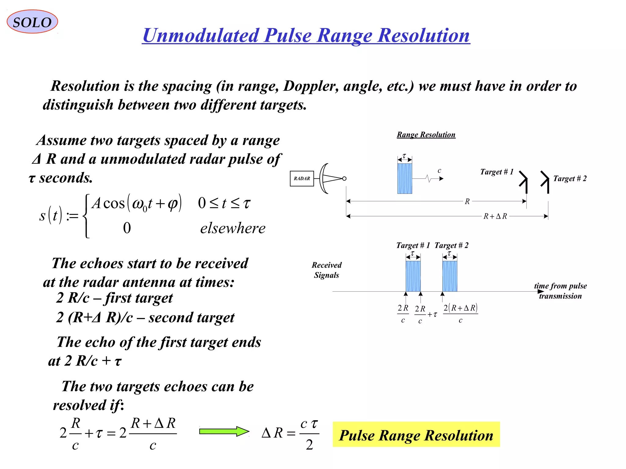
Explains resolution in RADAR systems, showing how to distinguish between targets based on signal strength and timing.
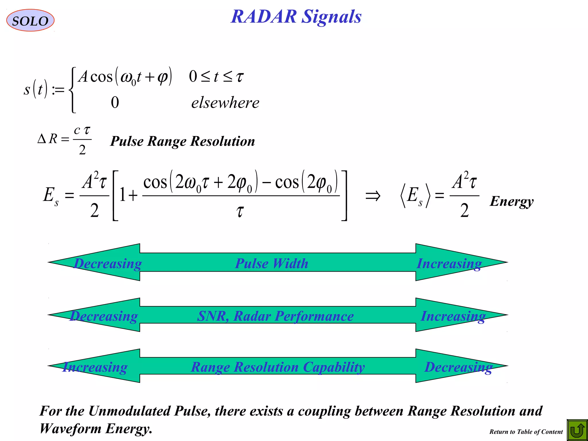
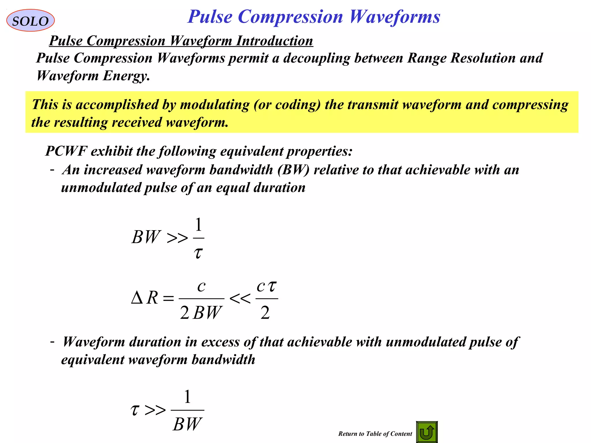
Discusses energy characteristics of unmodulated pulses in radar and introduces pulse compression waveforms.
Details various radar waveforms including CW radars and outlines the hierarchy based on modulation techniques.
Focuses on techniques used in pulse compression, emphasizing coding, modulation, and implementation hardware.
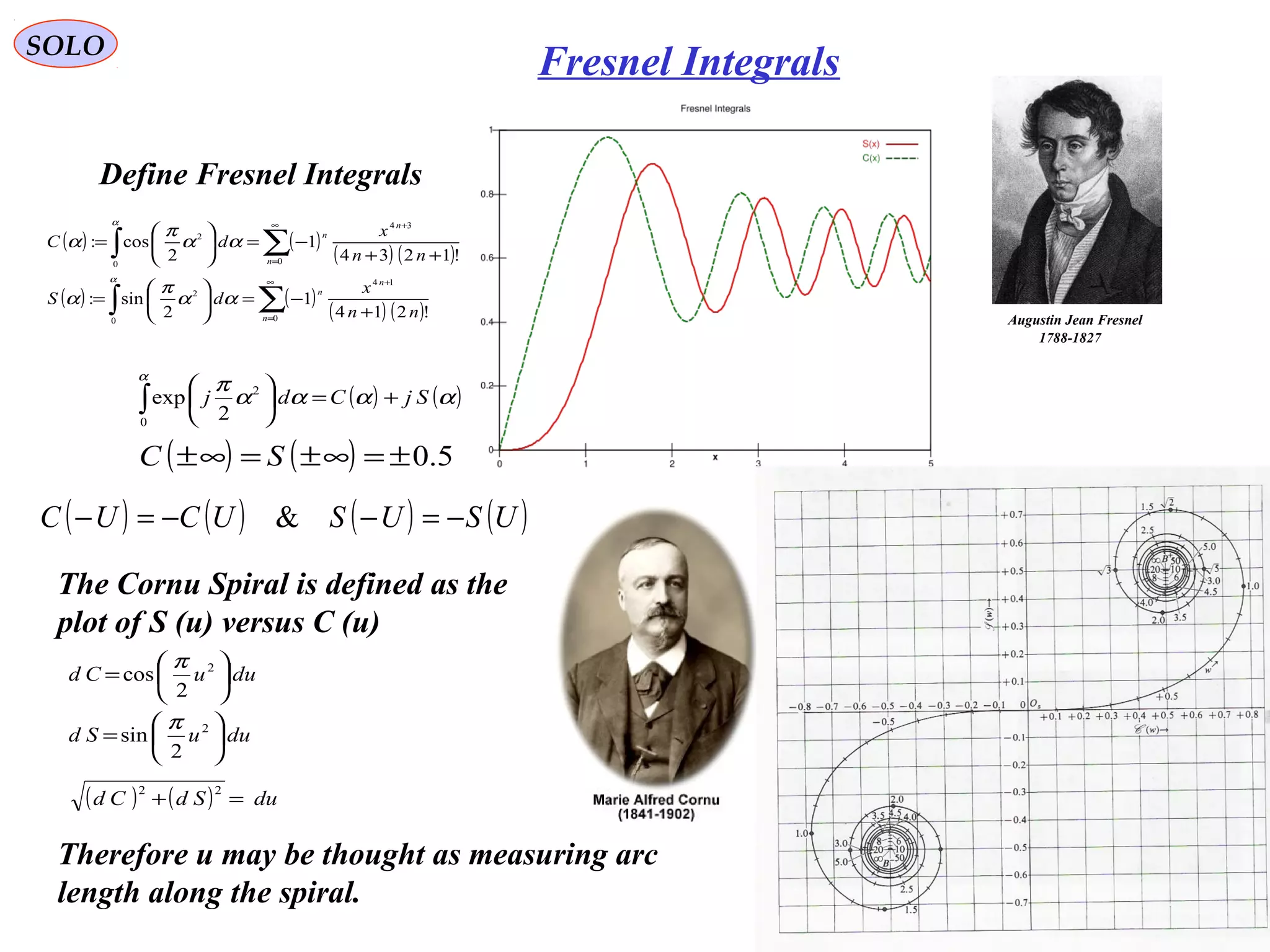
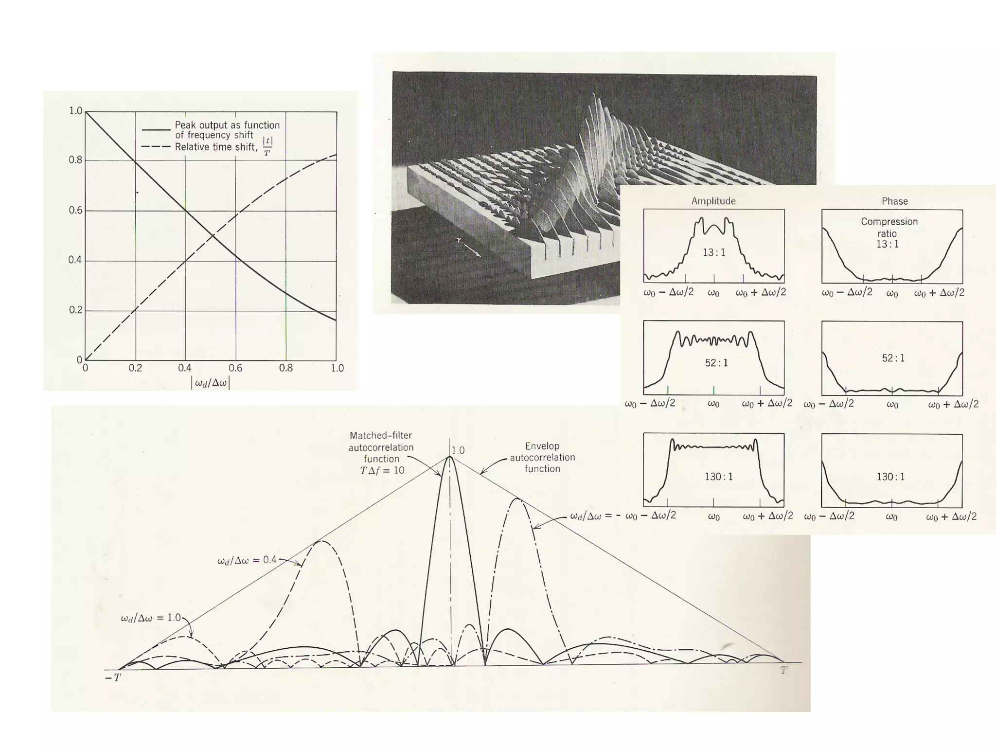
Details the linear FM modulated pulse technique, its Fourier transform, and characteristics of chirp and its applications.
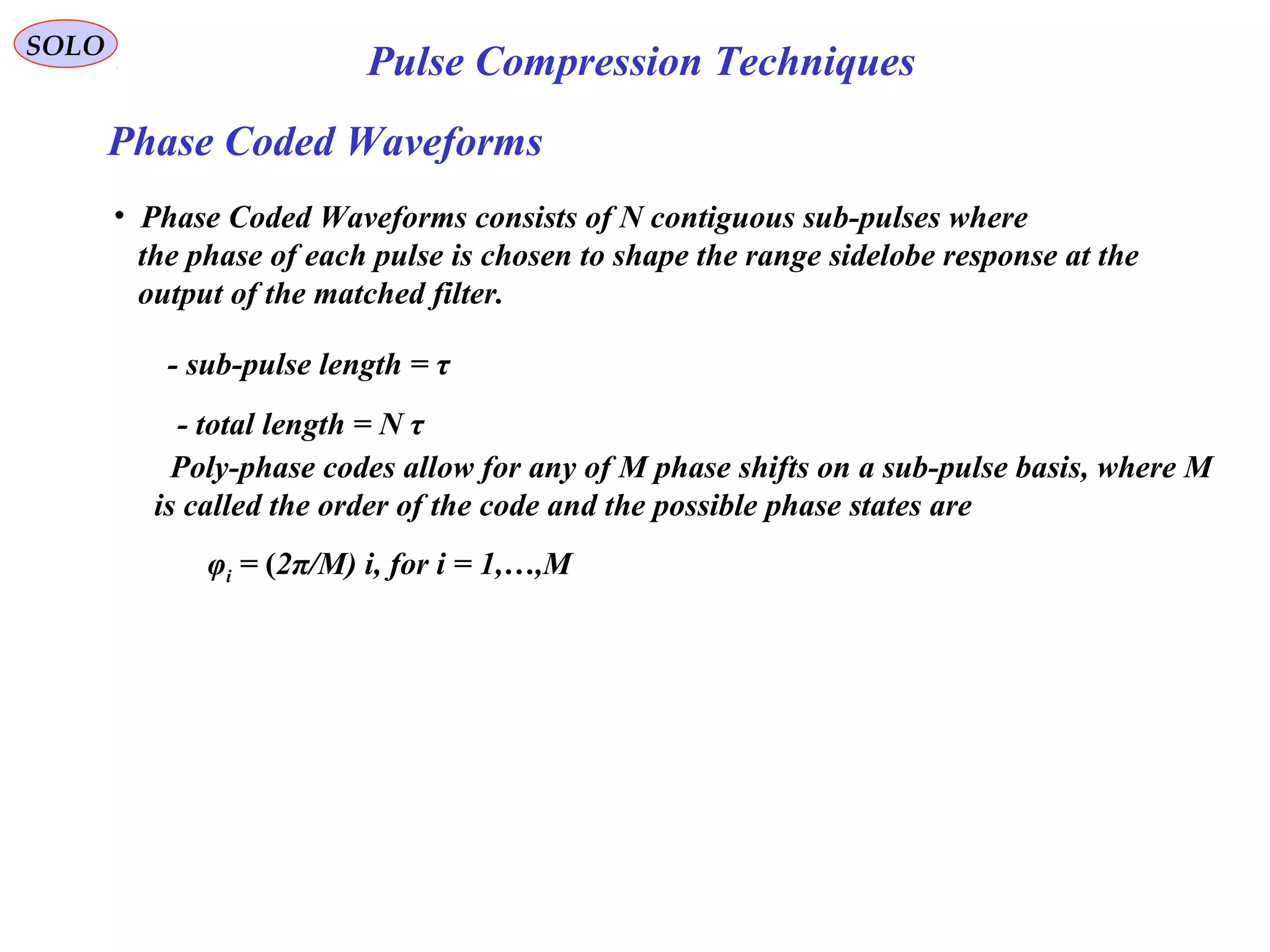
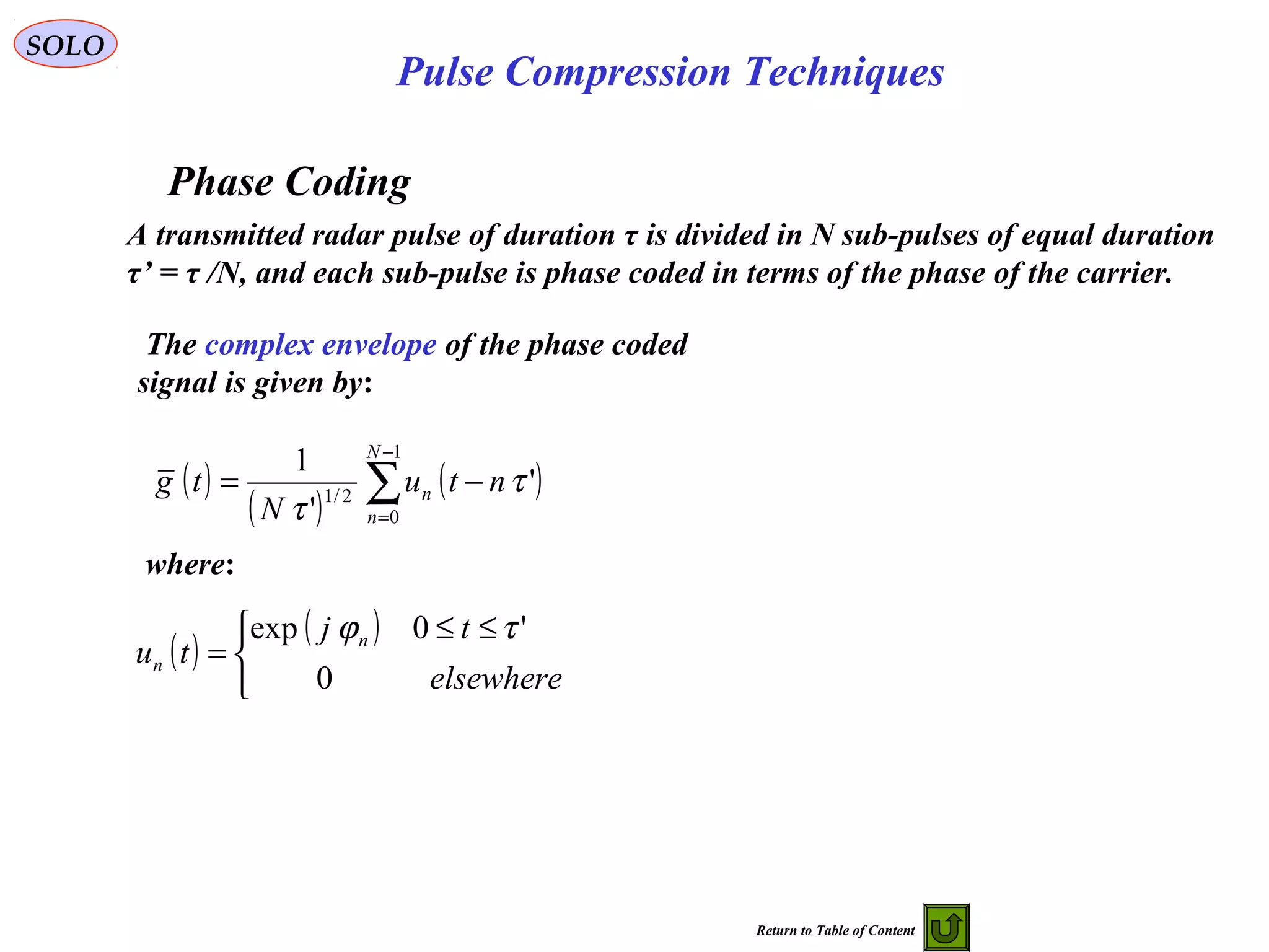
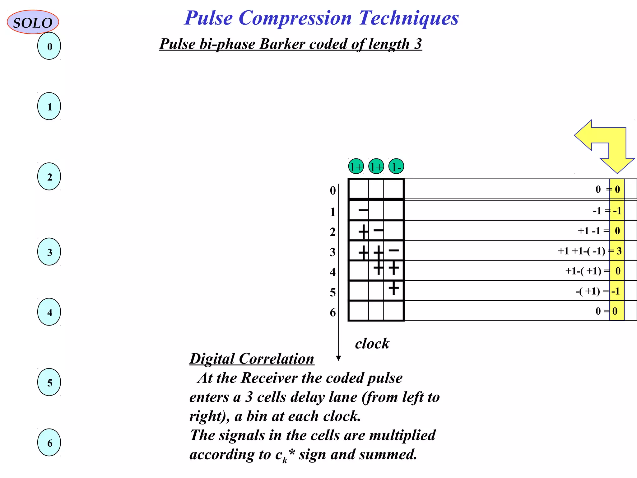
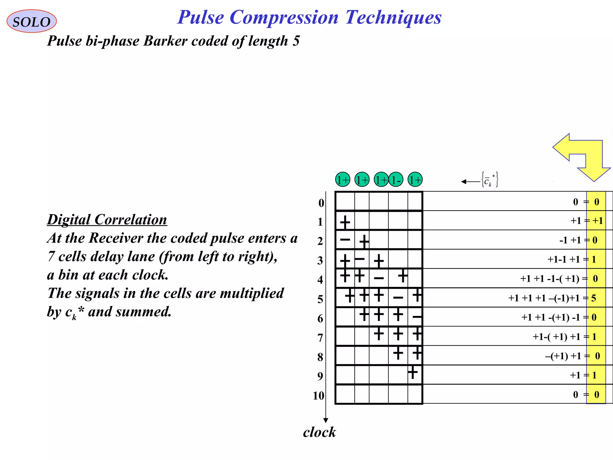
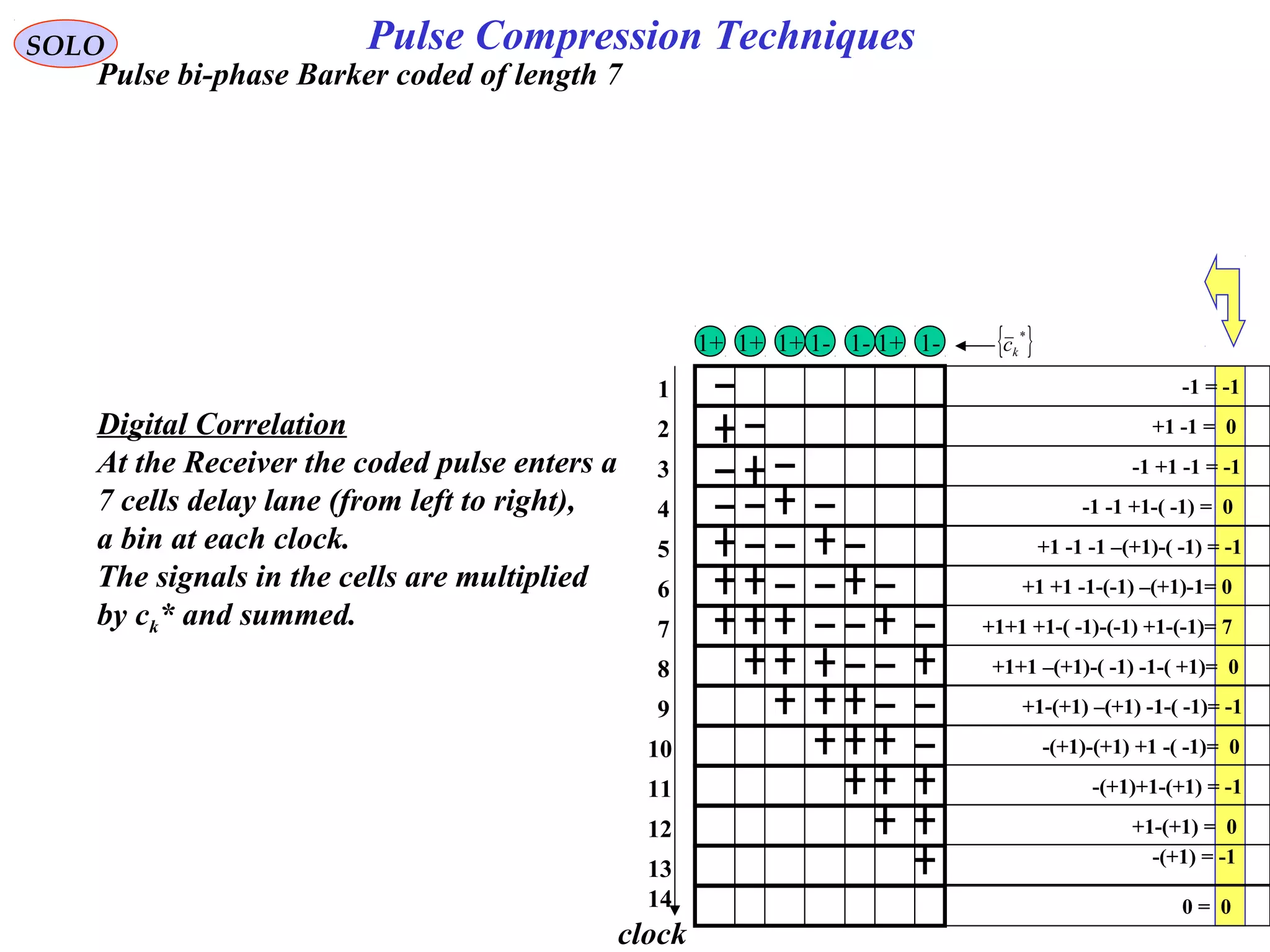
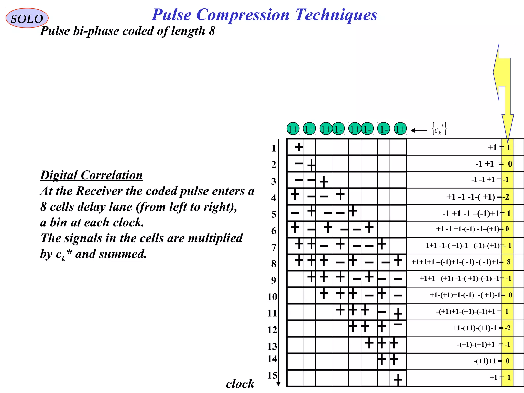
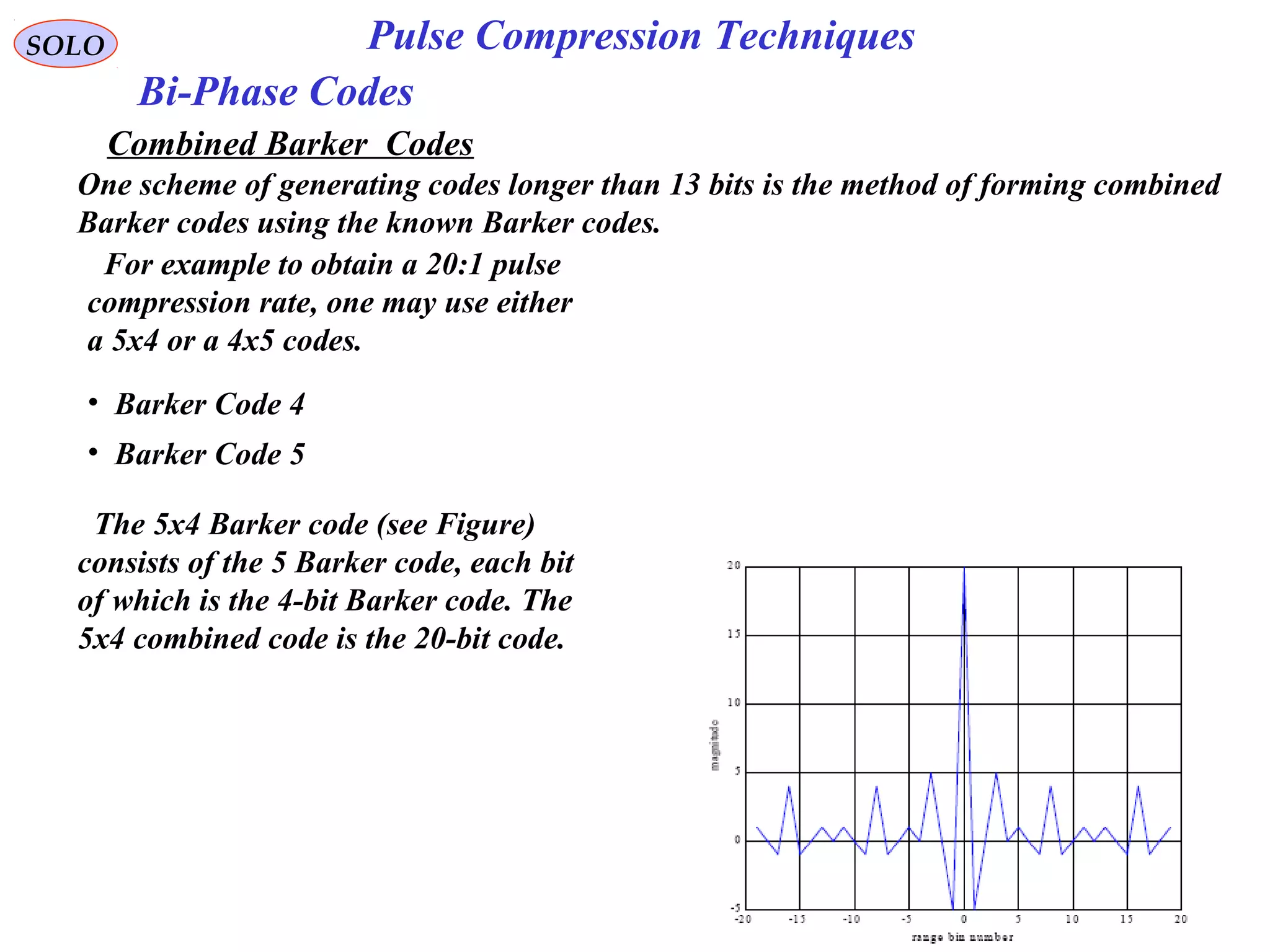
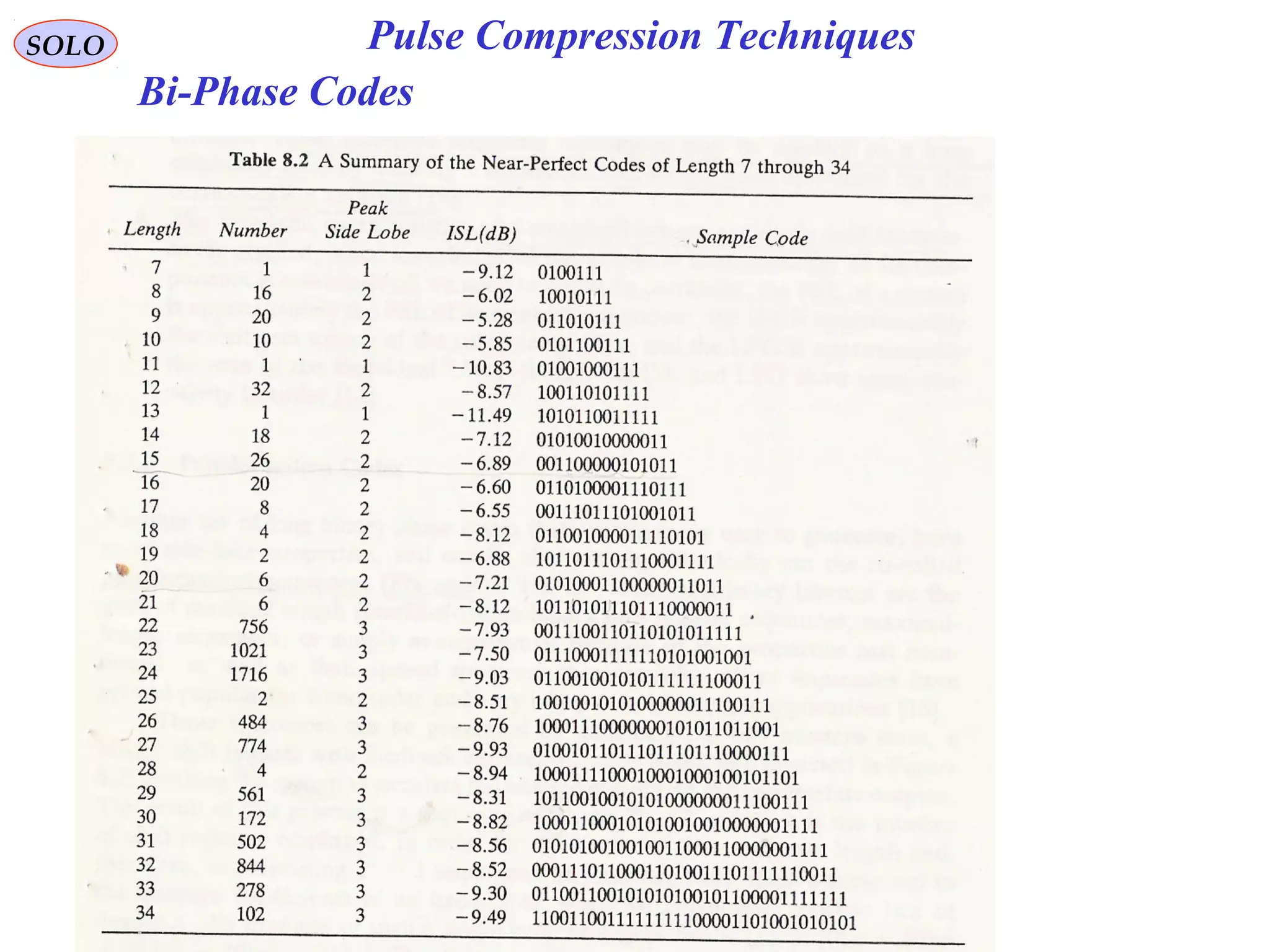
Explains phase-coded waveforms, including bi-phase codes and Barker codes, and their sidelobe characteristics.
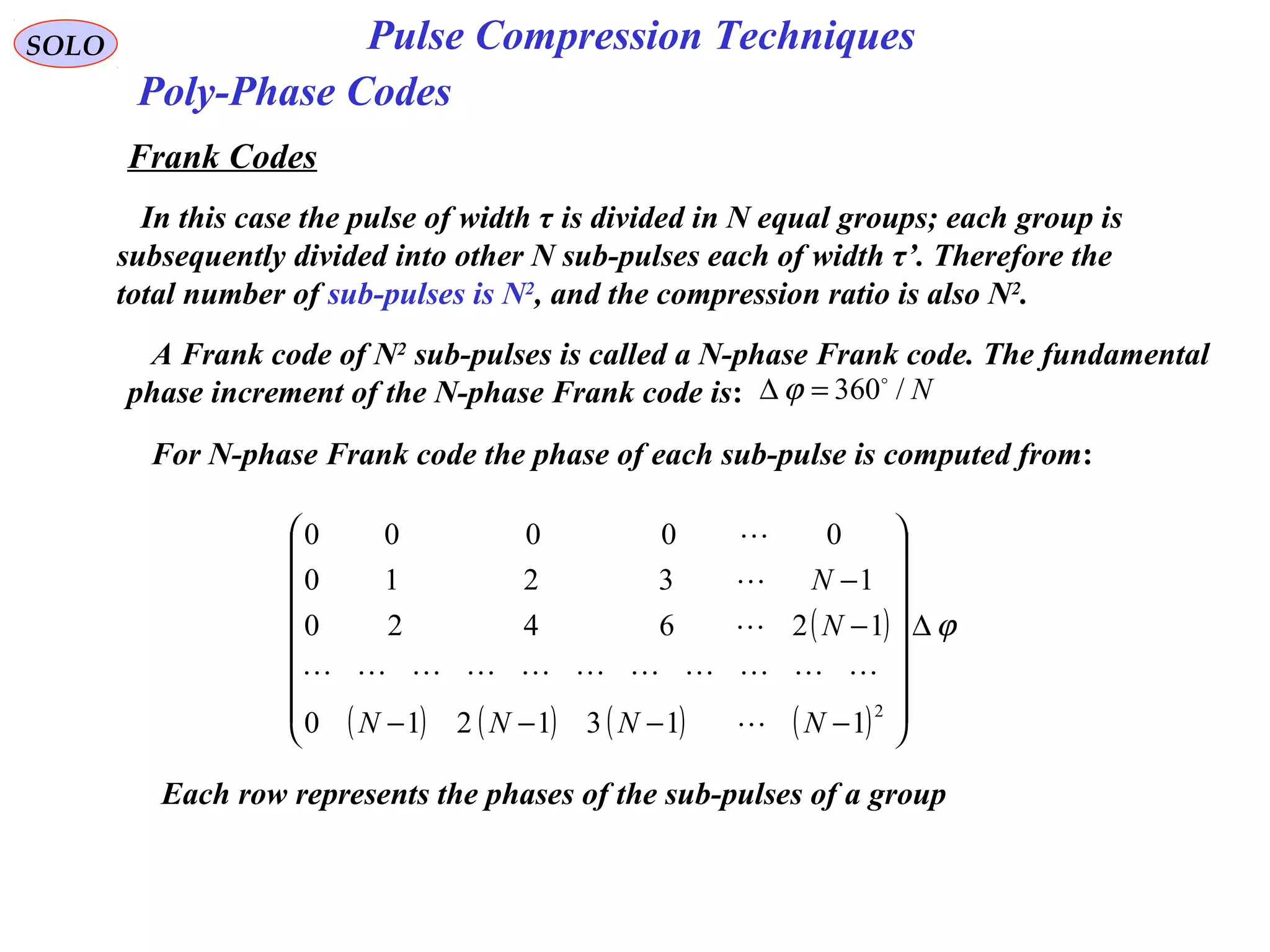
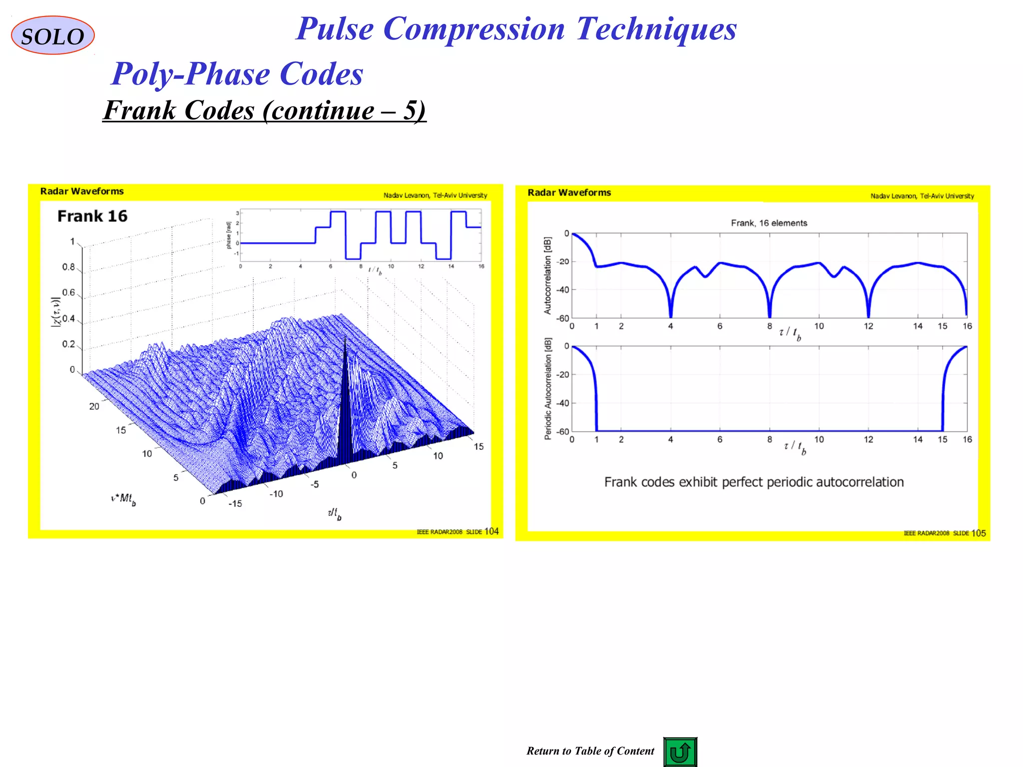
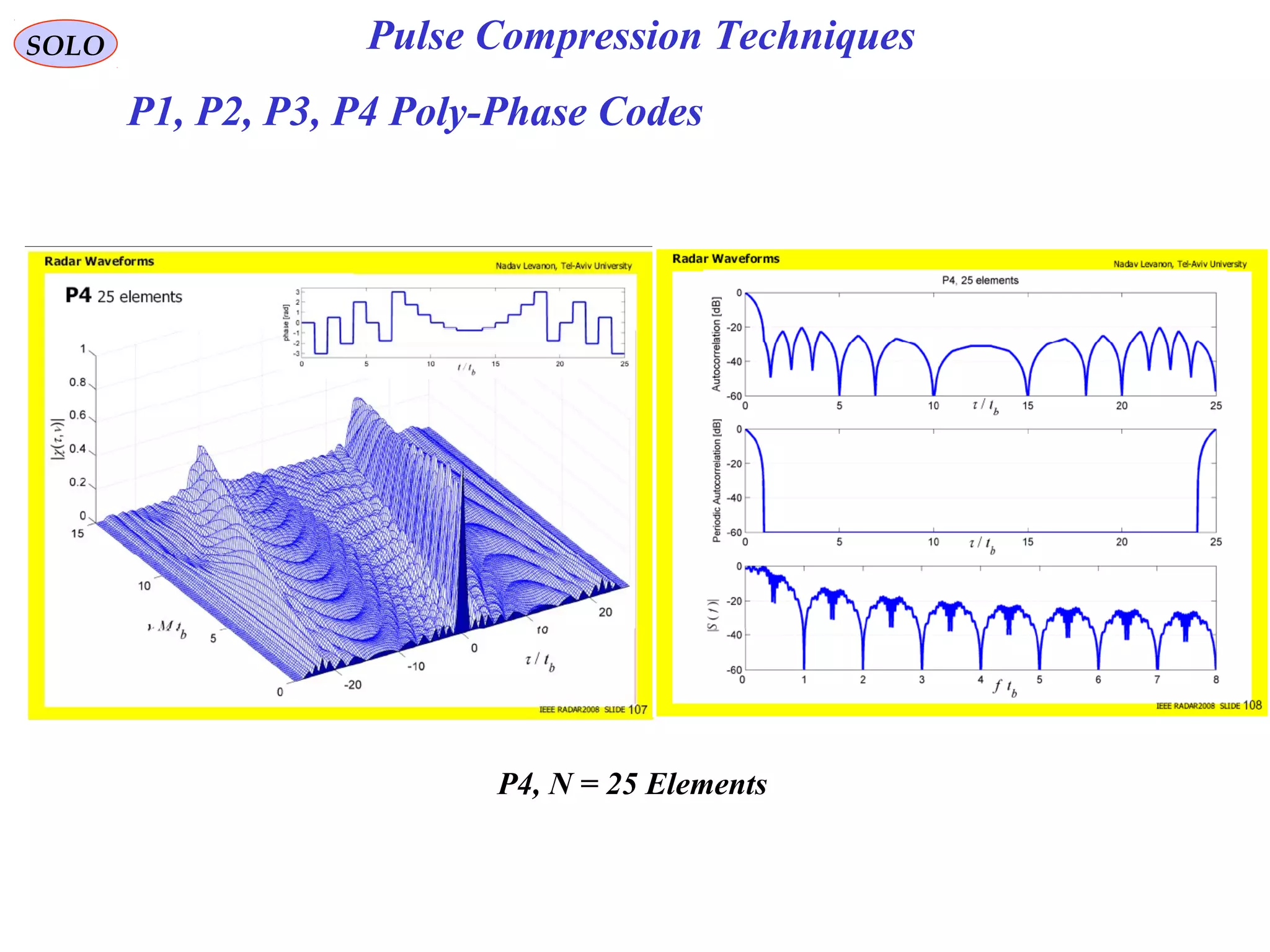
Describes poly-phase codes, Frank codes, and their applications in pulse compression with a summary of their benefits.
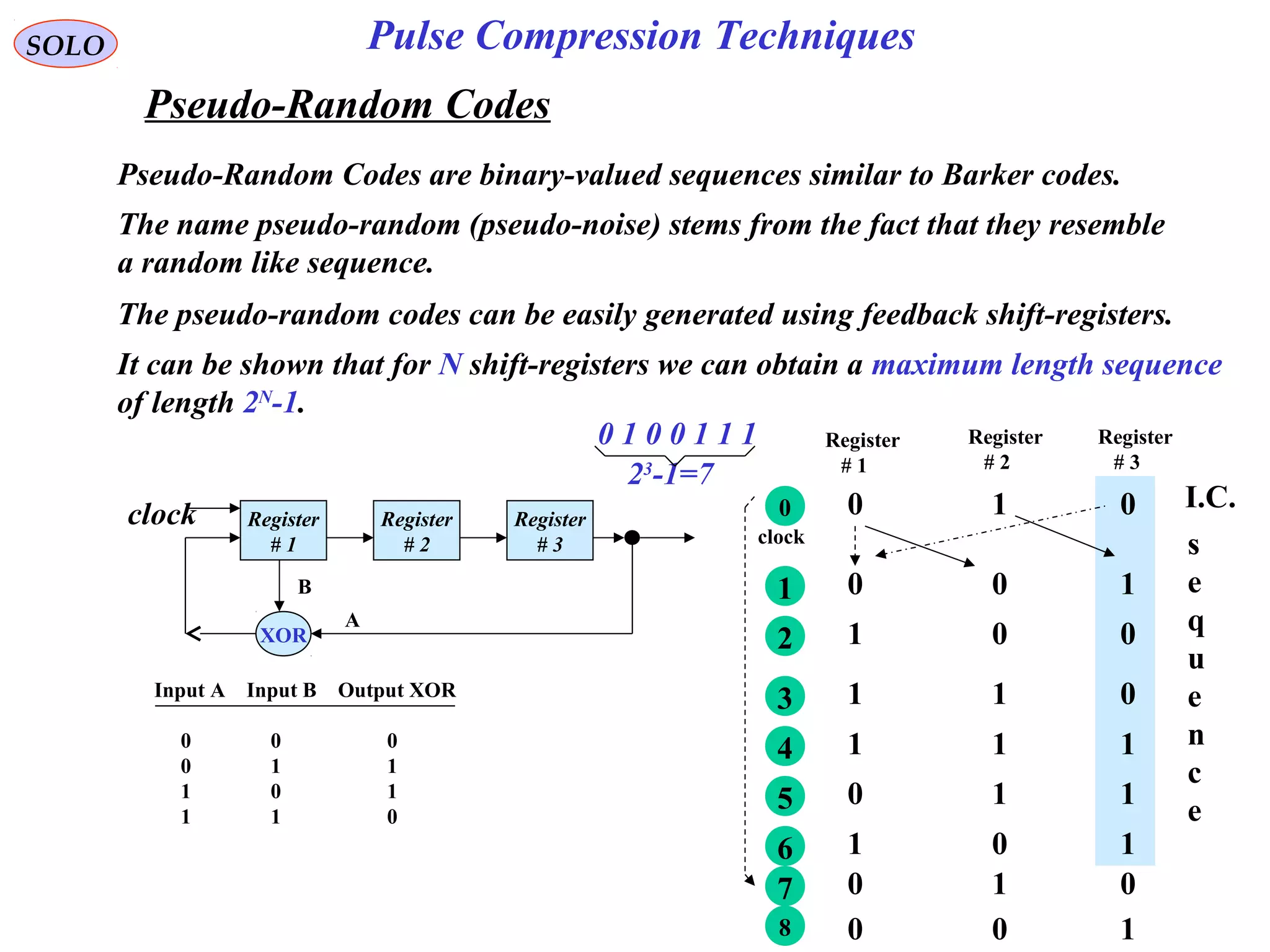
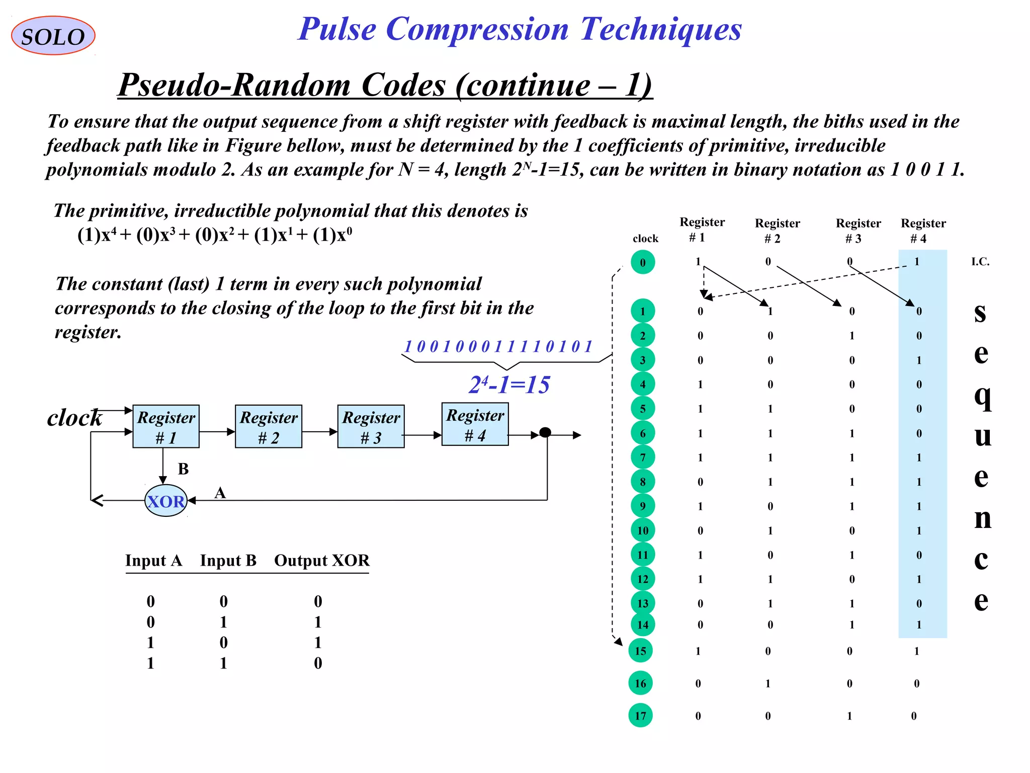
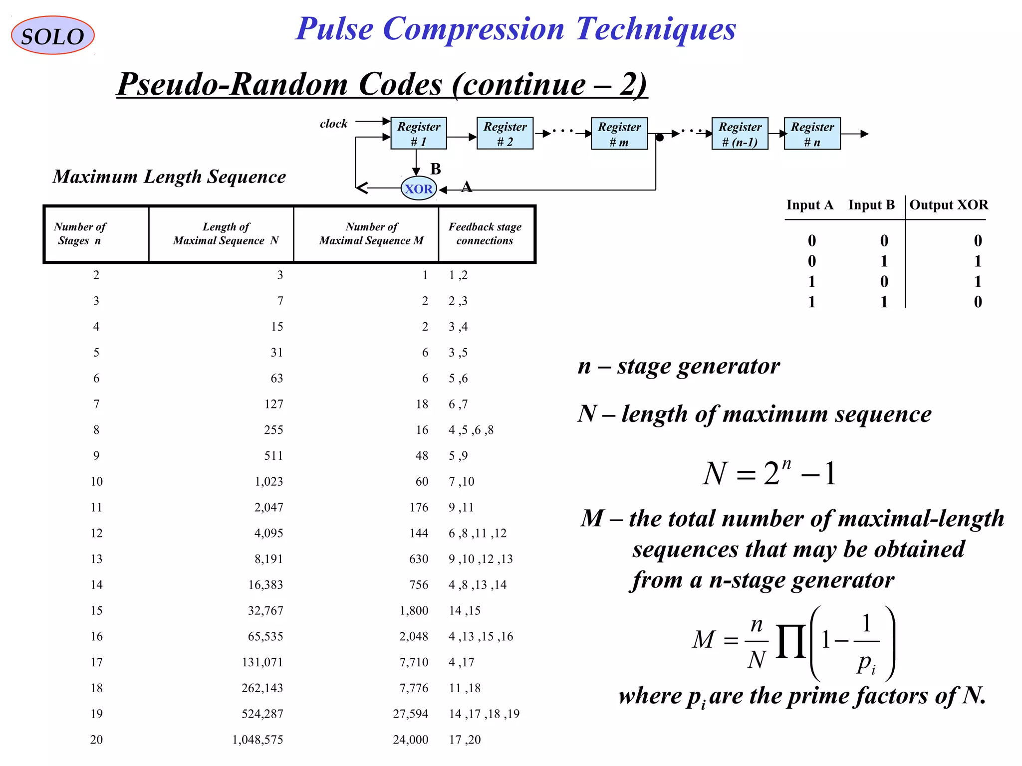
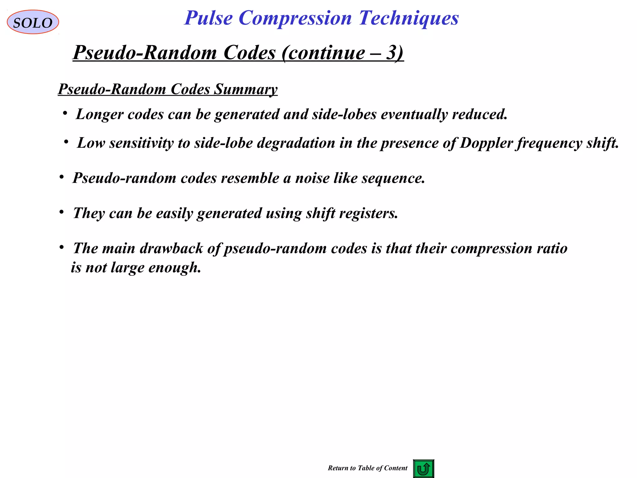
Discusses pseudo-random codes, their generation, properties, and limitations compared to other coding techniques.
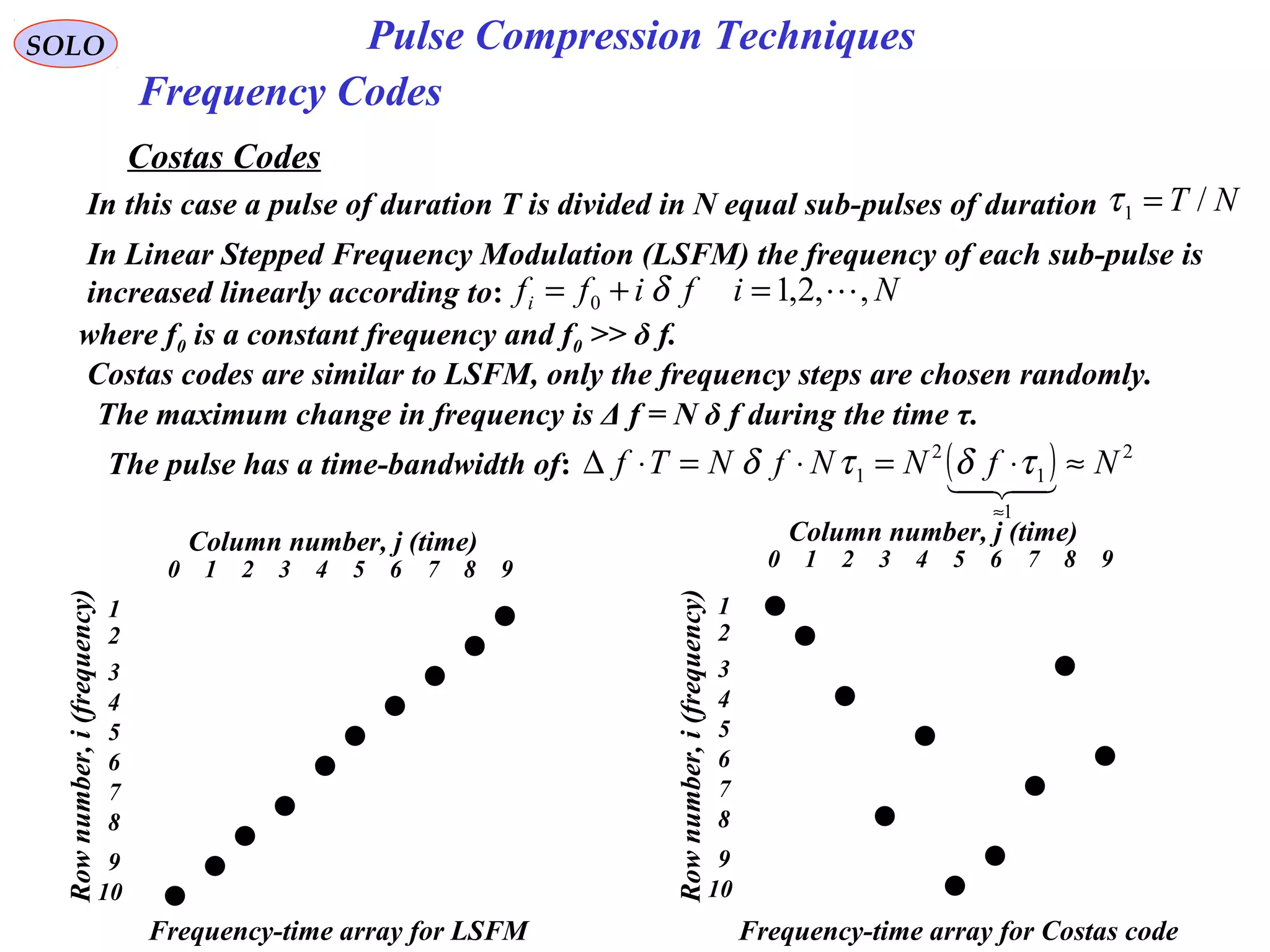
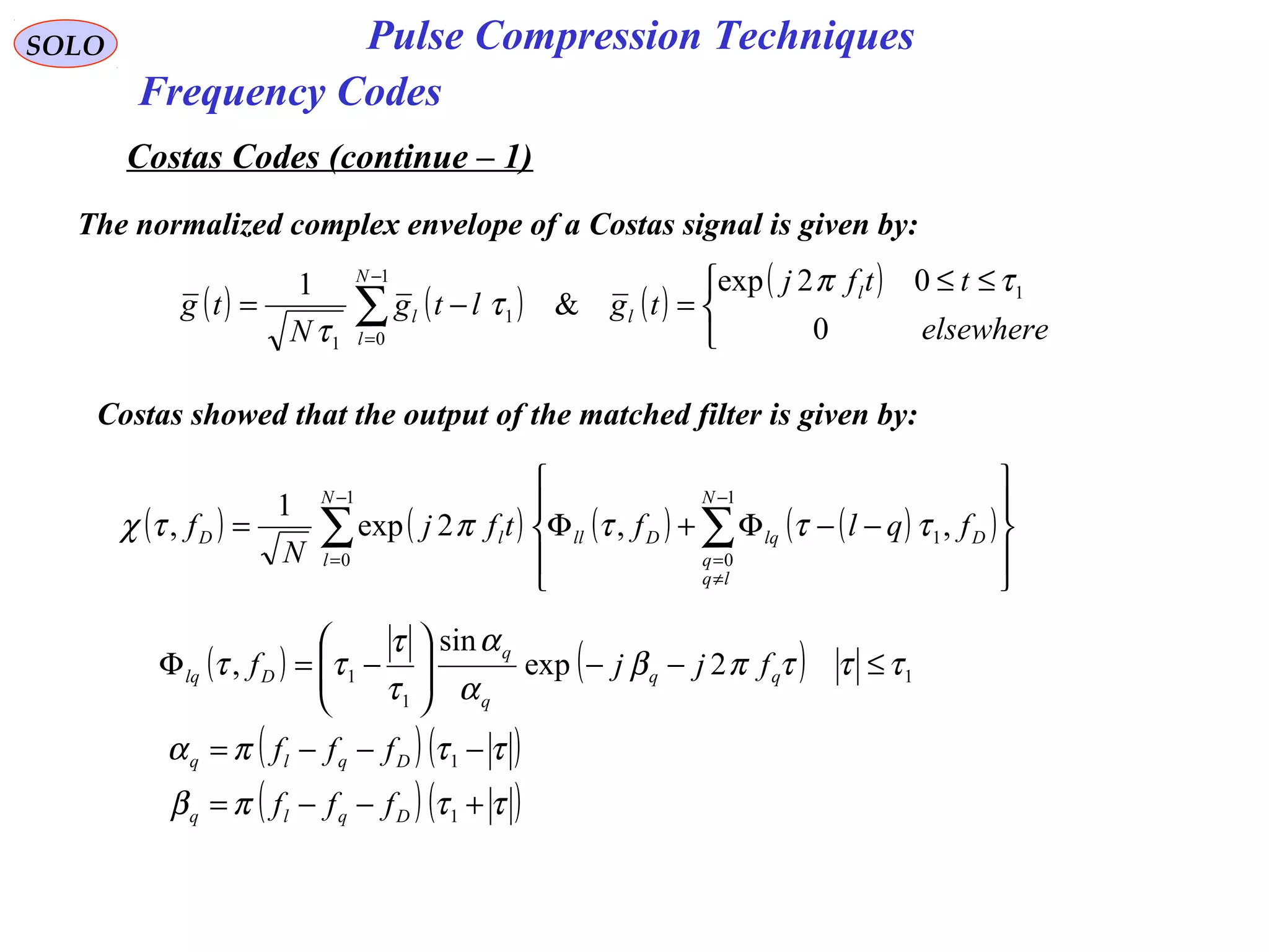
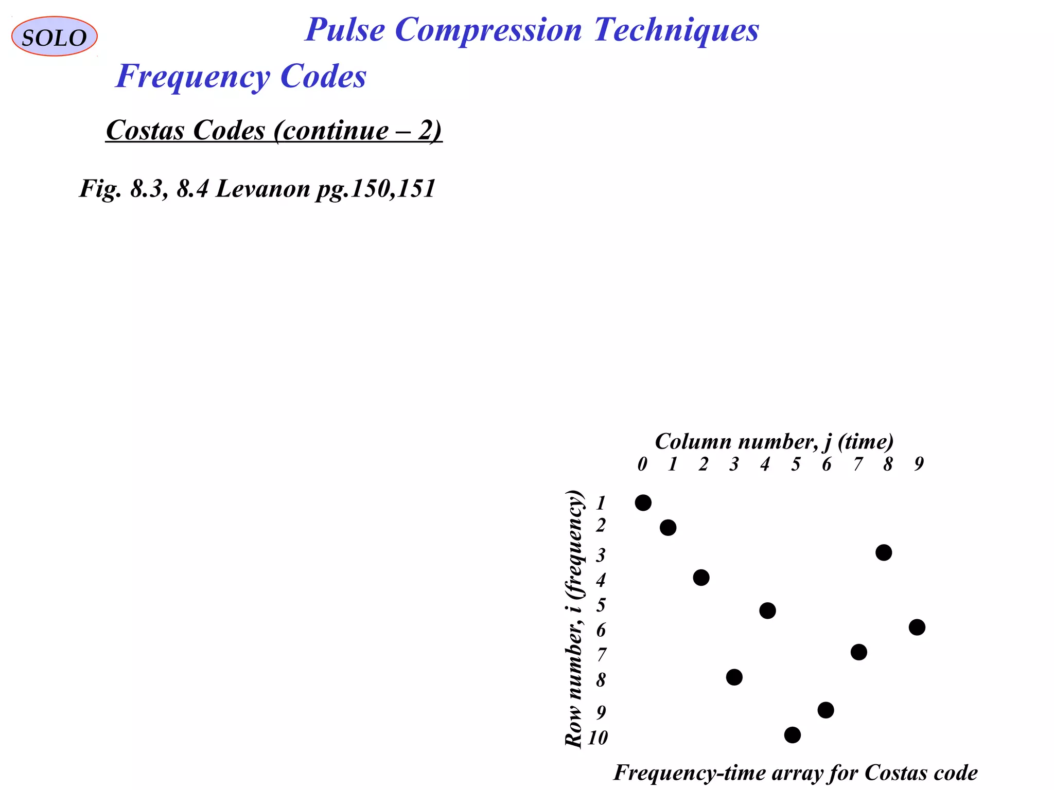
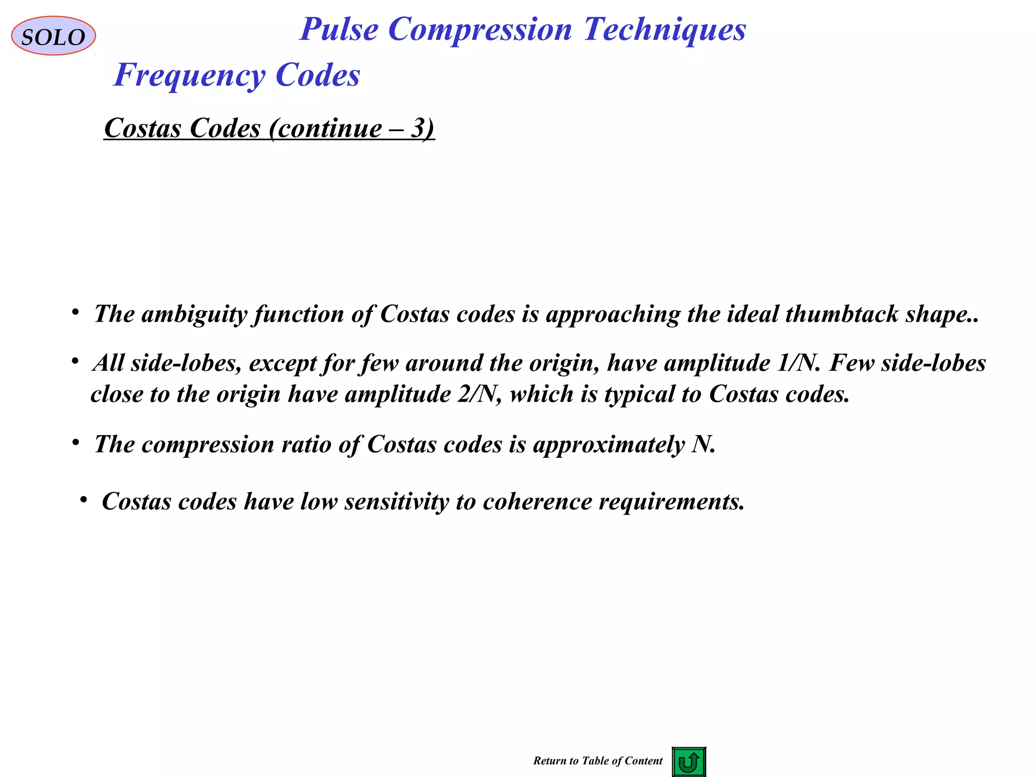
Explains frequency codes and Costas codes, their structures, and performance characteristics.
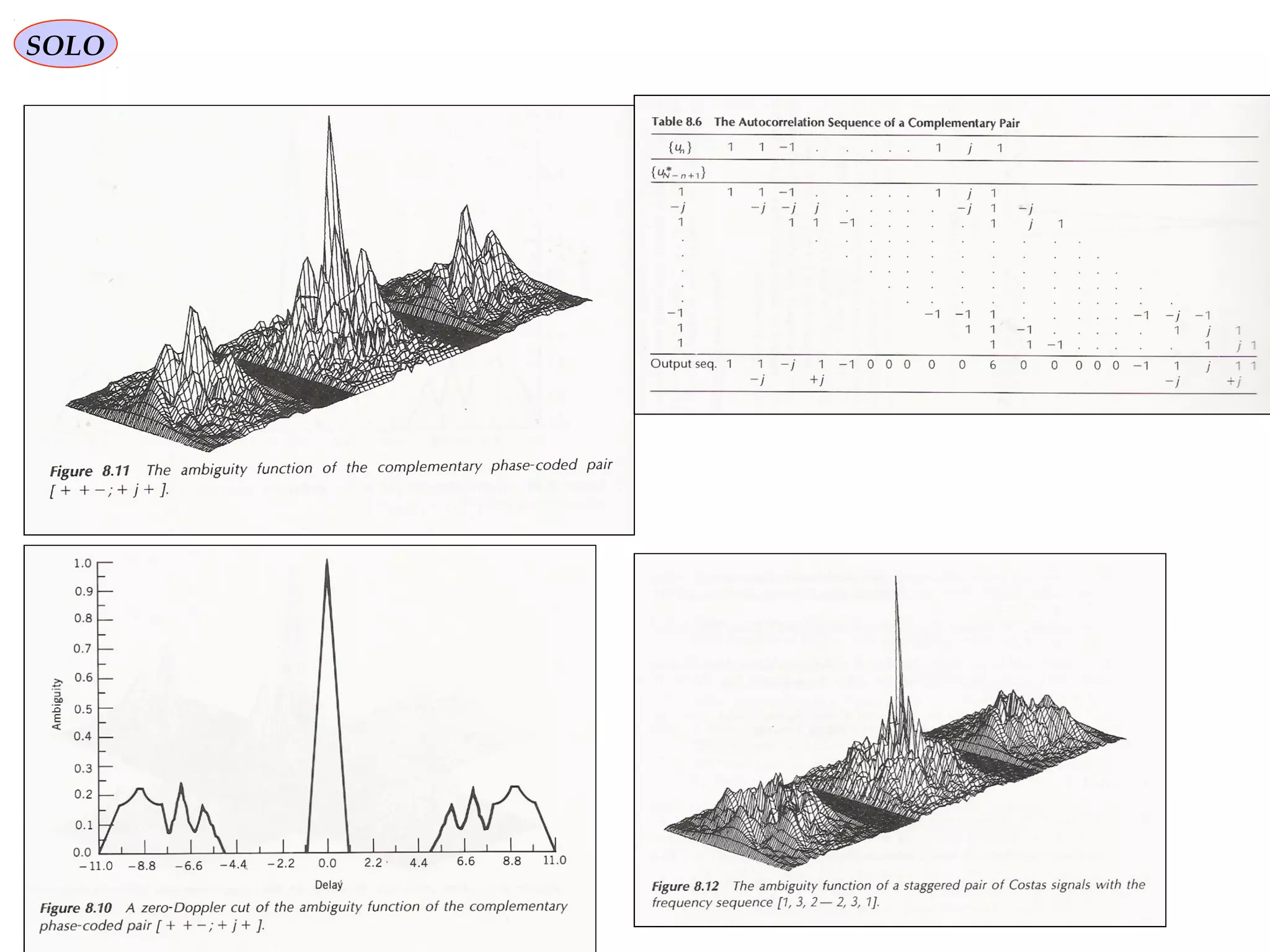
Introduces complementary pulse codes, providing references for further reading on radar principles and techniques.
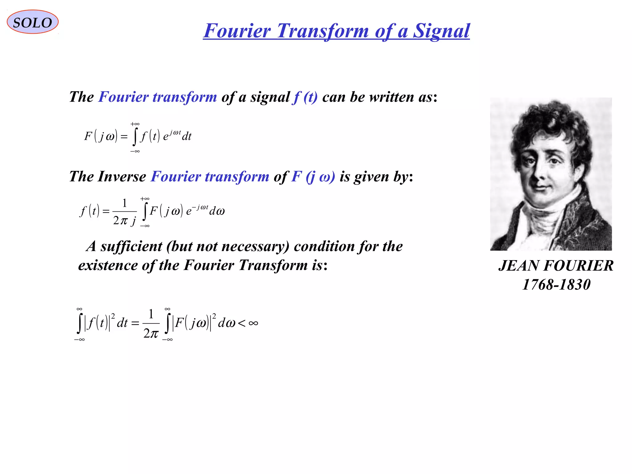
Discusses the Fourier transform's role in analyzing signals and waves in radar applications, including key formulations.