A Tutorial on Radar System Engineering

Dr LEE Kar Heng
Chief TBSS Group
Ph.D, M.Eng, M.Sc, B.Tech(Hons), MIEEE
Certified Teacher in Higher Education SEDA & TP
RADAR SYSTEM
ENGINEERING
IEEE International Conference on
Advanced Telecommunications
Conference, Ho Chi Minh City,
Vietnam, 2015

2
• The speaker is thankful to TERMA for the use of
TERMA Radar technical information in this
tutorial
• Terma has delivered 7 radars in Vietnam
– 2 Surface Movement Radars: Tan Son Nhat
International Airport and Noi Bai International
Airport
– 3 Vessel Traffic Radars: Port of Ho Chi Minh City
– 2 Vessel Traffic Radars: Port of Hai Phong
Acknowledgement

3
Tutorial Objective
• To understand the entire functionalities of radar
systems: its components and operations

4
Tutorial Outline
Scan Pattern
Generator
Antenna Duplexer
Waveform
Generator
Transmitter
Receiver
Signal
Processor
Data
Extractor
Data
Processor
Radar
Display
• A Typical Radar System

5
Quick Review
• RADAR- Radio Detection and Ranging
• Theory of reflection, absorption and scattering
• Higher frequency gives better result (???)
• Information from radar: Range, height, direction,
direction of motion, relative velocity

6
• Target distance is calculated from the total time (tdelay) taken by
the pulse to travel to the target and back to the radar
• c = 3 x 108 m/s, speed of light
Quick Review
tdelay

7
Quick Review
Video
Noise Noise & clutter Noise & clutter
tdelay

8
Quick Review
Noise
(not necessarily
visible)
Targets
(land)
Targets
(vessels)
Sea Clutter
Rain
VRM 63 km
(34 NM)
A weather
radar will see
rain clutter as
information.
A navigation
radar will see
rain clutter as
noise.

10
• Block diagram of a typical pulsed radar
A Pulsed Radar System
TX
RXAntenna
Motor
Motor Controller
Magnetron
Modulator
HV, PW
Receiver
Limiter
LNFE
IF Amplifier
Video Ampl.
STC
Video
Processing
Power
Supplies
Encoder, ARP & ACP’s
Control
Wave Guide
Circulator
Interface
Interface to external equipment

11
• A typical radar system
Antenna System
Transceiver
• Transmitter
• Receiver
• Plot Extractor
• Tracker
• Control
Electronics
• Interface
Two transceivers
provides
redundancy and
hot-standby

12
• The Transceiver:
WG SSPA
WG Assy
SSPA

13
• The Transceiver – Waveguide Assembly:
13

14
• The transmission:
WG
WG
Coupler
Limiter / STC
Adapter
Adapter
Transmission from antenna
SSPA
Signal coming from SSPA
enters the circulator
through WG SSPA
Signal passing the
circulator cw and
takes first exit
Signal enters the
antenna through
the installed WG

15
• The reception:
WG
WG
Coupler
Limiter / STC
Adapter
Adapter
Reflections from
targets are
captured by the
antenna
RxTx
Signal arrives coupler,
a -50 dB signal out for
measurement purposes
Signal passing the
circulator cw and
takes first exit
Signal enters the
circulator through
the installed WG
RxTx
Control
RxTx
Signal added through a
-20 dB coupler - for
calibration purposes
Attenuation of the
signal up to 40 dB
Test port
RxTx
Signal passing the
circulator cw and
applied the RxTx
module

16
• The antenna receives the EM energy from the
transmitter and radiates the energy into the free space
Antenna System
• An isotropic antenna radiates the
energy in a spherical pattern
• The energy is distributed equally
in all directions
16

17
Antenna System
• In practice, the radiated energy is focused in a
direction
• The radiation pattern describes how the energy
is radiated (or focused)
• The characteristics of radiation pattern are
beamwidth, gain and sidelobes
The ability to focus the
EM energy gives the
gain of the antenna

18
Antenna System
• Radiation from a directional source
• The energy is focused in a given
directions
• This allows the energy to travel
further, hence a gain, G,
compared to the isotropic
source
18

19
Antenna System
• Coastal Surveillance and Vessel Traffic System radars are
usually fan or inverse-cosecant-squared beams
fan beam pattern
Inverse-cosecant-square beam pattern

20
Antenna System
• A 21’ Slotted Waveguide Array Antenna

21
Antenna System
• Horn directs the EM energy and hence improves the
antenna gain (1)
• The polarization filter gives circular or horizontal
polarization (3)
• The antenna is protected by a
radome (4)
• The antenna is radiated by the
slotted waveguide (2)
Radome (front)
Horn
Polarization filterRF radiator
(slotted waveguide)
Radome (back)
1
2 3
44 1

22
Antenna System
• The beam pattern: beamwidth

23
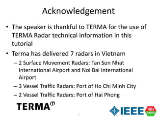
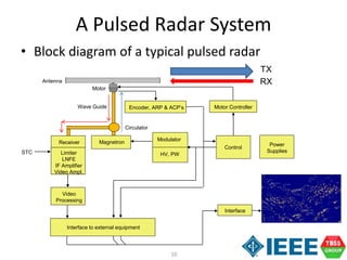
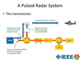
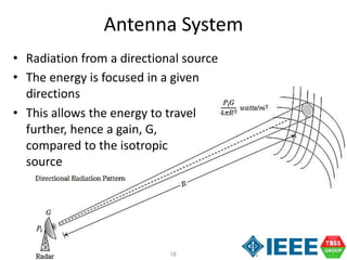
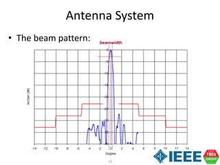
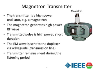
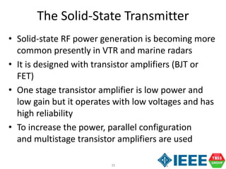
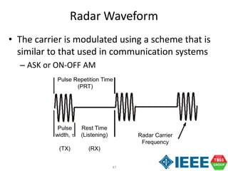
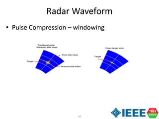
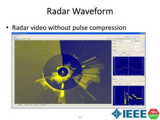
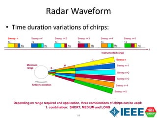
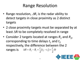
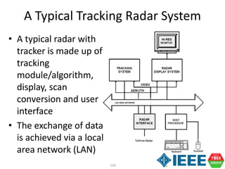
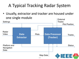
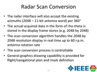
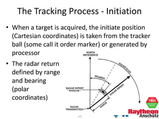
Antenna System
• Antenna performance:
Main Parameters:
Frequency band 9.14 - 9.47 [GHz]
VSWR
9.345 - 9.405 GHz ≤ 1.15
9.140 - 9.470 GHz ≤ 1.20
Gain ≥ 38 [dBi]
Integrated Cancellation Ratio ≥ 15 [dB]
Azimuth Pattern:
Horizontal BW @ -3 dB ≤ 0.35 [º]
Side lobe level
± 1.5º to ± 5º ≤ -28 [º]
± 5º to ± 10º ≤ -30 [º]
Exceeding ± 10º ≤ -35 [º]
Elevation Pattern:
Elevation beam form Fan
Vertical BW @ -3 dB ≤ 11 [º]
Min. coverage @ -30 dB -18 [º]
Tilt (fixed) -1.5 [º]

24
Antenna System
• For mechanically-steered antenna, the bearing
information is obtained using encoder
Antenna
A B C
A
B
C
Direction
(encoder)

25
Antenna System
Radome
Encoder Assembly and Rotatory Joint Module
Linear
array
Antenna
Tx
Rx
Flared horn
Connection
box
Power
Encoder(s)
Thermal
sensors
Encoder (s)
Rotary joint
Waveguide
RF Flange
Turning unit
Gearbox
Thermal
sensors
Motor
Antenna unit
Slotted waveguide (SWG)

26
Antenna System
• The encoder:
ENCODER
Stationary Waveguide Entry
(to transceiver)
Rotating Waveguide Entry
(to Antenna)
ENCODER INTERNAL

27
Antenna System
• The encoder:
Channel A
Channel A
Channel B
Channel B
Channel N
Channel N
photodetector
LED light
source
Rotating encoder disk,
gray or Manchester
coded generate the
counting pulse
Bipolar pulses
(RS422)

28
Antenna System
• Whenever a stationary waveguide is to be connected to
a rotating antenna, a rotating joint must be used
• In radars, rotary joints connect transmitter and/or
receiver to its rotating antenna
• A circular waveguide is normally used in a rotating joint
Stationary
Waveguide Entry
(to transceiver)
Rotating Waveguide
Entry (to Antenna)

29
Control
• It consists of a timing control that generates the
synchronization timing signals
Timing
Control
Modulator and
Transmitter
Receiver
Signal
Processor
Duplexer Antenna
To other
modules
Scan Pattern
Generator
(RPM, Beam
Control, …)

30
Modulator
• The modulator produces a high power DC pulse to the
transmitter
• A modulated signal is generated and sent to the antenna by the
modulator and transmitter block
• A train of narrow rectangular shaped pulses modulating a sine
wave carrier is transmitted
Pulse
width
Pulse Repetition Time
(PRT)
Rest Time
(Listening)
Radar Carrier
Frequency
30

31
Magnetron Transmitter
• The transmitter is a high power
oscillator, e.g. a magnetron
• The magnetron generates high power
RF wave
• Transmitted pulse is high power, short
duration
• The EM wave is sent to the duplexer
via waveguide (transmission line)
• Transmitter remains silent during the
listening period
Magnetron

32
Magnetron Transmitter
• The two main limitations of magnetron are
– Limited average power
– Poor ability to detect moving targets in heavy clutter
• The peak power of several MW can be produced by
magnetron, but the average power is limited to 1 -2
kW
• The pulse width limitation prevents the magnetron
from being used with pulse compression where
frequency or phase modulation is difficult
• Magnetrons are noisy outside the operating
frequency

33
Marine Radar Magnetrons
• The magnetrons have been used extensively in civil
marine radars
• They are compact and can generate peak powers
between 3 and 75 kW with average powers from a
few W to a few 10s of W
• They offer reliability which sea-goers require
• Marine radar operates at a fixed frequency within
the band 9.38 GHz to 9.44 GHz

34
Marine Radar Magnetrons
• A RF assembly that houses
both the transmitter and
receiver Magnetron
Circulator LNFE
TR Limiter
IF AMP
Assembly

35
The Solid-State Transmitter
• Solid-state RF power generation is becoming more
common presently in VTR and marine radars
• It is designed with transistor amplifiers (BJT or
FET)
• One stage transistor amplifier is low power and
low gain but it operates with low voltages and has
high reliability
• To increase the power, parallel configuration
and multistage transistor amplifiers are used

36
• The advantages of Solid State Transmitter
– Individual solid-state devices have long MTBF
– Maintenance is easy with modular design and
construction of solid state
– Broad bandwidth
– No cathode heating required (no need for high
voltage and warm up time)
– No pulse modulator required
– Solid-state transistor amplifiers have low noise and
good stability

37
• Advantages of Solid-State radars over magnetron radars
PARAMETERS SOLID-STATE MAGNETRON
Maintenance Low High – annual magnetron
replacement
Remote Control
and Monitoring
Fully digital and remote
controller
Requires digital interface
for full remote control
Built-in-Test (BIT) Extensive and fully remote
accessible
Limited
MTBF 50,000 hours 3,000 hours
Antenna Speed Electronically selectable,
high speed scanning gives
improved track quality
Standard 24 rpm, requires
motor and gear
replacements

38
• Advantages of Solid-State radars over magnetron radars
PARAMETERS SOLID-STATE MAGNETRON
Antenna Tilt Yes No
Emitted Power
Density
Low power mode for short
range use and operations
near hot ordinance
High
Variable Frequency Yes – electronic control No
Start-Up Instantaneous operation Warm up time
Spares Low High (replace magnetrons)
Frequency diversity
(improved
performance)
Yes No
Doppler processing Yes No

39
• Meeting IEC 60963-1/62388 Requirements
Height
(m)
RCS
(m2)
IEC 60936-1 (nm) IEC 623880 (nm) Solid-State
(nm)*
60 50000 20 20 24.2
6 5000 7 8 12.7
3 2500 --- 6 10.4
10 50000 7 11 15.6
5 1800 --- 8 11.6
4 7.5 --- 5 7.8
3.5 10 2 4.9 7.6
3.5 5 --- 4.6 7.2
2 2.5 --- 3.4 5.8
1 1 --- 2 4.1

40
• The parameters of a solid-state radar
PARAMETERS
X-BAND
S-BAND
Model 1 Model 2
Overall length 3.7 m 5.5 m 3.9 m
Turning circle diameter 3.8 m 5.6 m 4 m
Frequency band 9.22 – 9.44 GHz
Gain 32.7 dB 34.5 dB 27.5 dB
Horizontal beamwidth 0.7 0.45 2 max.
Vertical beamwidth 2 2
Horizontal sidelobes
within 10
-26 dB At least -28
dB dowm
Horizontal sidelobes
outside 10
-33 dB At least -35
dB down

41
• The detection performance of the X-band radar:
Antenna
Height
Target
Type
Modeled as fluctuating point
target
Detection and Tracking distance
(nm)
RCS (m2) Height (m) Clear Weather 10 mm/h Rain
50 m
AMSL
1 1 1 m AMSL 10/8.25 (SS4) ----
2 3 2 m AMSL 12/11.23 (SS5) 9/10.64 (SS 5)
3 10 3 m AMSL 14/13.3 (SS6) 12/12.71 (SS6)
4 100 5 m AMSL 17/16.29 (SS7) 15/15.83 (SS7)
5 1000 8 m AMSL 20/19.2 (SS8) 18/18.71 (SS8)
• The results are obtained from CARPET based
on PFA = 10–6 and PD = 80%

42
• A Typical Transmitter Design based on SSPA
SSPA
WG
Assy
RxTx
BP
BP
BP
BP
Combiner
1300 MHz
7825 MHz (VTS)
7600 MHz (SMR)
1300 MHz 7825 MHz (VTS)
7600 MHz (SMR)
9.225 - 9.5 GHz (VTS)
9.0 - 9.275 GHz (SMR)
TxRAM/FPGA
DAC /
DDS
DAC /
DDS
BP
BP
AttenuationAttenuation
RxTx Control
100 - 375 MHz (low)
100 - 375 MHz (high)

43
A Typical Solid-State Transmitter
• The design of a solid-state transmitter:
Power
Amplifier
Power
Amplifier
Module 1
Module 2
Powersplitter
Poweradder
Incomingsignal
Transmittedsignal

44
• The solid-state power amplifier (SSPA) amplifies
the signal before transmission
• The transmitted power ranges from 50 W (short
range) to 200 W (long range) typically
• The required power is constructed using multi-
stage and parallel configuration of single stage
power amplifiers PA module
In Out
8 W power transistor
50 W power amplifier

45
• The typical solid-state power amplifier
50 W
200 W

46
• The degradation performance
0%
10%
20%
30%
40%
50%
60%
70%
80%
90%
100%
0%
25%
50%
75%
100%
Percentage of power transistors in failure
Available SSPA power
Output power
Free space range

47
Radar Waveform
• The carrier is modulated using a scheme that is
similar to that used in communication systems
– ASK or ON-OFF AM
Pulse
width, t
(TX)
Pulse Repetition Time
(PRT)
Rest Time
(Listening)
(RX)
Radar Carrier
Frequency

48
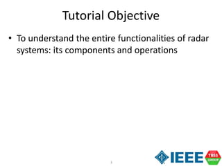
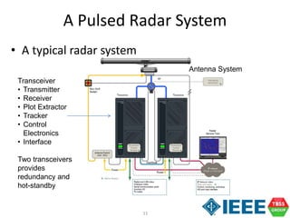
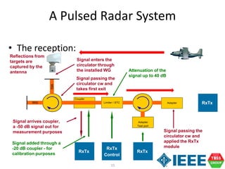
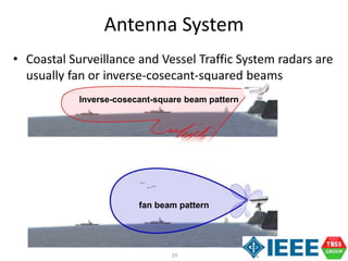
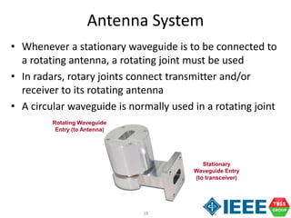
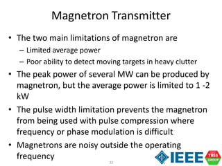
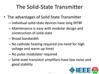
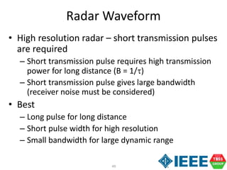
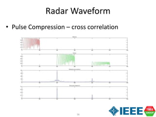
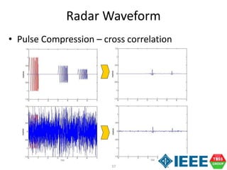
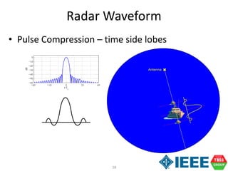
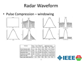
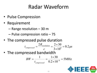
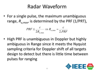
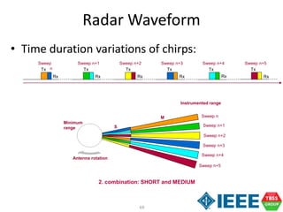
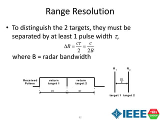
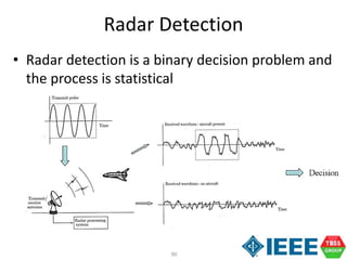
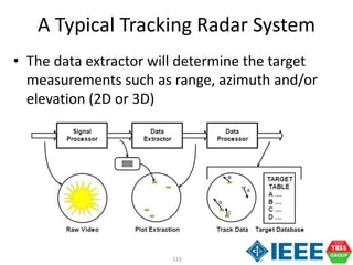
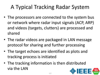
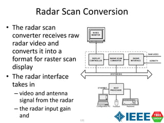
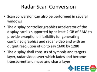
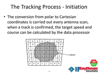
Radar Waveform
• The Chirp Pulse:
Time
Amplitude
Time
Frequency
f [MHz]
1 2 3 4 5 6
Chirp BW Separation
Time
Amplitude
Time
Frequency
or
35 Mhz 6 Mhz
f [MHz]
100 375
f [MHz]
100 375
1300 MHz
7825 MHz
(VTS)
7600 MHz
(SMR)
100 - 375 MHz
1400 - 1675 MHz
9225 - 9500 MHz (VTS)
9000 - 9275 MHz (SMR)
9260 9301 9342 9383 9424 9465
9441.5
9447.5

49
Radar Waveform
• High resolution radar – short transmission pulses
are required
– Short transmission pulse requires high transmission
power for long distance (B = 1/t)
– Short transmission pulse gives large bandwidth
(receiver noise must be considered)
• Best
– Long pulse for long distance
– Short pulse width for high resolution
– Small bandwidth for large dynamic range

50
Radar Waveform
• The signal flow:

51
Radar Waveform
• Pulse Compression
Every little part of the wave
represents a specific frequency
Low frequencies
are slowed down
High frequencies
are speeded up
Processing

52
Radar Waveform
Transmitted chirp
Received chirp

53
Radar Waveform
f1f2f3f4
Σ
Σ
Σ
f1
f2
f3
f4
Σ
Bandpass Delay Summation

54
Radar Waveform
f1f2f3f4
f1
f2
f3
f4

55
Radar Waveform
Σ
Σ
Σ

56
Radar Waveform
• Pulse Compression – cross correlation

57
Radar Waveform
• Pulse Compression – cross correlation

58
Radar Waveform
• Pulse Compression – time side lobes
Antenna

59
Radar Waveform
• Pulse Compression – windowing

60
Radar Waveform
• Pulse Compression – windowing

61
Radar Waveform
• Requirement
– Range resolution – 30 m
– Pulse compression ratio – 75
• The compressed pulse duration
• The compressed bandwidth
s
c
R
t resolution
compressed 2.0
103
3022
8




MHz5
102.0
3011
6



 
compressedt
BW

62
Radar Waveform
• Requirement
– Range resolution – 30 m
– Pulse compression ratio – 75
• The required transmission pulse width
• If the SSPA gives 200W, the virtual transmitted
power
kW1575200  PCRPP SSPAvirtual
sPCRtcompressed t 1575102.0 6
 

63
Radar Waveform
• Radar video with pulse compression

64
Radar Waveform
• Radar video without pulse compression

65
Radar Waveform
• For a single pulse, the maximum unambiguous
range, Ru,max, is determined by the PRF (1/PRT),
• High PRF is unambiguous in Doppler but highly
ambiguous in Range since it meets the Nyquist
sampling criteria for Doppler shift of all targets
design to detect but there is little time between
pulses for ranging
PRF
c
R
R
c
PRF u
u .22
max,
max,


66
Radar Waveform
• Medium PRF radar may be
ambiguous in both Doppler and
range since it samples too fast for
echoes from long range but too
slow to Nyquist sample the Doppler
shift of all targets
• Medium PRF however has the best
of both worlds, a compromise
performance between unambiguity
in Doppler and range
• Low PRF is unambiguous in range
but high ambiguous in Doppler
since it waits until the last
transmitted pulse arrives before the
next transmission
Low PRF
t
PRT = 1/PRF
f
0 PRFPFF
High PRF
t
f
0 PRFPFF

67
Radar Waveform
• Different PRF is used in different application such as
Low PRF or Medium PRF is suitable for detection of
vessels while High PRF is used in detecting air targets
• Careful selection of PRF will also result in better tracking
performance since one must be able to detect a target
before tracking it
• Mixture of pulse durations enhances the performance

68
Radar Waveform
• Time duration variations of chirps:
Rx
Tx
Rx Rx Rx
Tx Tx Tx Tx
Rx
Tx
Rx
Sweep n Sweep n+1 Sweep n+2 Sweep n+3 Sweep n+4 Sweep n+5
t
Instrumented range
Minimum
range
Antenna rotation
S
M
L Sweep n
Sweep n+1
Sweep n+2
Sweep n+3
Sweep n+4
Sweep n+5
Depending on range required and application, three combinations of chirps can be used:
1. combination: SHORT, MEDIUM and LONG

69
Radar Waveform
Rx
Tx
Rx Rx Rx
Tx Tx Tx Tx
Rx
Tx
Rx
Sweep
n
Sweep n+1 Sweep n+2 Sweep n+3 Sweep n+4 Sweep n+5
Instrumented range
Minimum
range
Antenna rotation
S
M Sweep n
Sweep n+1
Sweep n+2
Sweep n+3
Sweep n+4
Sweep n+5
2. combination: SHORT and MEDIUM

70
Radar Waveform
Rx
Tx
Rx Rx Rx
Tx Tx Tx Tx
Rx
Tx
Rx
Sweep
n
Sweep n+1 Sweep n+2 Sweep n+3 Sweep n+4 Sweep n+5
t
Instrumented range
Minimum
range
Antenna rotation
S Sweep n
Sweep n+1
Sweep n+2
Sweep n+3
Sweep n+4
Sweep n+5
3. combination: SHORT only

71
• The receiver amplifies the radar returns and prepares them
for signal processing
• Extractor of target information from the returns is
performed by the signal processor, tdelay is determined for
each detected target
• Target distance is calculated from the total time (tdelay) taken
by the pulse to travel to the target and back
c = 3 x 108 m/s, speed of light
1 s = 300,000,000 m
= 300,000 km
1ms = 300 km
Target Range

72
Target Range
The PRF determines how often the radar transmits (PRF = pulses/s =
1/PRT or 1/PRI) and the maximum range of the system (PRT = Pulse
Repetitive Time, PRI = Pulse Repetitive Interval)
Transmitted
pulses
Pulse travels 150 km in 0.5 ms
Maximum range = 0.25 ms (75 km)
Echo needs 0.25 ms to return
Transmitted
pulses
Pulse travels 300 km in 1 ms
Maximum range = 0.5 ms (150 km)
Echo needs 0.5 ms to return
PRF = 2 kHz
PRT = 0.5 ms
PRF = 1 kHz
PRT = 1 ms
1 ms

73
Average Power
• In each cycle (PRT), the radar only radiates from
t sec (known as pulse width or PW)
• The average transmitted power is
where Pt = peak transmitted power and
PRF = Pulse Repetition Frequency,
. .av t tP P P PRF
PRT
t
t
 
  
 
1
PRF
PRT


74
Range Ambiguity
• The range that corresponds to the 2-way time delay is
the radar unambiguous range, Ru
• Consider detection of 1 target at R1 in two separate
transmissions
Transmitted
Pulses
Received
Pulses
Pulse 1 Pulse 2
echo 1 echo 2
PRT
t
tdelay
tdelay
Ru
(R )
1
R2

75
Range Ambiguity
• Echo 1 is the return from target at range R1,
• Echo 2 is the return from the same target at
range R1, from the 2nd transmission
• Echo 2 can also be taken as an echo from a
different target from the 1st transmission
1
2
delayct
R 
2 1
2
delayct
R R 
 
2
2
delayc PRT t
R

 ERROR!!!

76
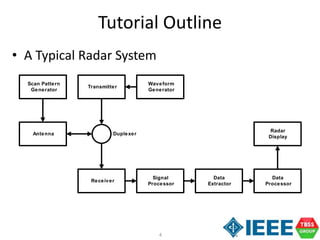
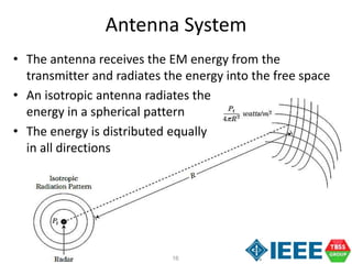
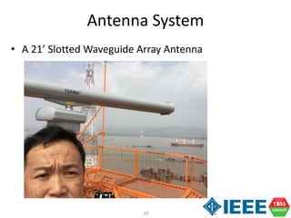
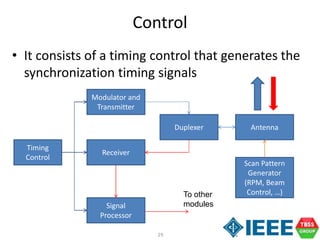
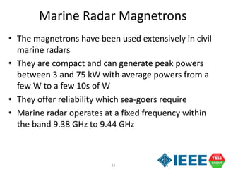
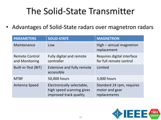
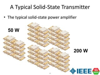
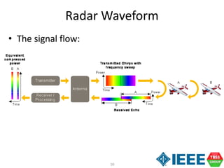
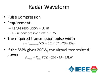
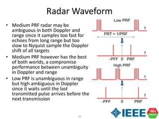
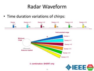
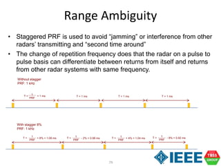
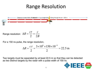
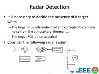
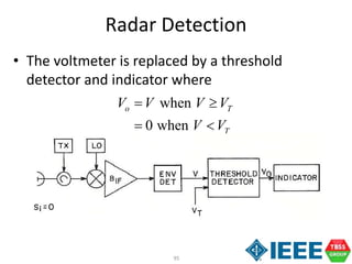
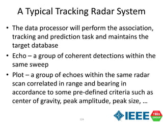
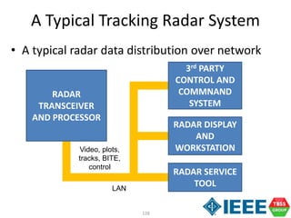
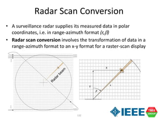
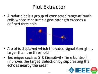
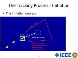
Range Ambiguity
• The maximum unambiguous range: ,max
2 2
u
cPRT c
R
PRF
 Page 2 of 4
Range: 5 NM
Transmit
Pulse 1
t = 0 Next pulse
Time needed for the pulse to hit the target: T = 31 µs
Time needed for the pulse to return to the antenna: T = 31 µs
Time needed between two pulses: T > 62 µs or PRF < 16.1 kHz (corresponding 2 x range, here 10 NM)
Target at 5 NM
t = 31 µs
Receive
Pulse 1
t = 62 µs
PRF [Hz]
1000
1500
2200
4000
8000
[km]
150
100
68.2
37.5
18.7
Max. range [NM]
81
54
36.8
20.2
10.1
300.000 km/s
300.000 km/s
Max. range =
c
2PRF
150.000
PRF
81.000
PRF
km NM
76

77
Range Ambiguity
The illustration of range ambiguity using lattice diagram:
t
PRF 3.75 kHz, T = 266.7 µs
30 km
T = 266.7 µs
Tx pulse n
Tx pulse n+1
Tx pulse n+2
Tx pulse n+3
40 km
T = 266.7 µs
T = 266.7 µs
T = 266.7 µs
RANGE 40 km
Tx pulses
Echoes 30 km
Echoes 60 km
Range
60 km
200 µs
200 µs
200 µs
200 µs
133.3 µs
133.3 µs
133.3 µs

78
Range Ambiguity
Falsetarget
Truetarget
T0
t-n
t
t-n
t
t-n
t
t-n
t
T0Sweep 1
T0Sweep 2
T0Sweep 3
T0Sweep 4
Falsetarget
Truetarget
T0AND
T0ADD

79
Range Ambiguity
• Staggered PRF is used to avoid “jamming” or interference from other
radars’ transmitting and “second time around”
• The change of repetition frequency does that the radar on a pulse to
pulse basis can differentiate between returns from itself and returns
from other radar systems with same frequency.
T =
1
PRF
Without stagger
PRF: 1 kHz
= 1 ms T = 1 msT = 1 ms T = 1 ms
T =
1
PRF
With stagger 8%
PRF: 1 kHz
+ 8% = 1.08 ms T =
1
PRF
- 2% = 0.98 ms T =
1
PRF
+ 4% = 1.04 ms T =
1
PRF
- 8% = 0.92 ms

80
Range Ambiguity
T0
Falsetarget
t-n t-m t-p t-q
Truetarget
t t t t
Falsetarget
Truetarget
T0
T0
T0
T0
Sweep 1
Sweep 2
Sweep 3
Sweep 4
AND T0
ADD T0

81
Range Resolution
• Range resolution, R, is the radar ability to
detect targets in close proximity as 2 distinct
targets
• 2 close proximity targets must be separated by at
least R to be completely resolved in range
• Consider 2 targets located at ranges R1 and R2,
corresponding to time delays t1 and t2
respectively, the difference between the 2
ranges is  2 1 2 1
2 2
c c
R R R t t t     

82
Range Resolution
• To distinguish the 2 targets, they must be
separated by at least 1 pulse width t,
where B = radar bandwidth
2 2
c c
R
B
t
  
Received
Pulses
return
target 1
c
return
target 2
t ct
target 1 target 2
ct

R R1 2

83
2 2
c c
R
B
t
  
Range Resolution
Range resolution:
Pulse width = 1 µs, length of pulse flying through the air = 300 mDistance is half of 300 m = 150 m
For a 150 ns pulse, the range resolution,
m5.22
2
10150103
2
98




tc
R
Two targets must be separated by at least 22.5 m so that they can be detected
as two distinct targets by the radar with a pulse width of 150 ns.

84
Range Resolution
PW: 1 μs
Length: 300 m
Range resolution: 150 m
150 m
120 m
PW: 250 ns
Length: 75 m
Range resolution: 37.5 m
50 m
30 m
PW: 50 ns
Length: 15 m
Range resolution: 7.5 m
10 m
7 m

85
• The number of wavelengths contained in the two way path
between the radar and the target,
• Total phase shift,
• Radar is able to give radial velocity
of a moving target from Doppler
Effect
• Doppler effect causes a shift in
frequency of the received echo
signal from a moving target
• Doppler frequency shift
• Let R be the Range of the target
Doppler Effect
RADAR TOWER
INBOUND
ECHO
RADAR
ANTENNA
TRANSMIT
PULSE
OUTBOUND
ECHO
2R
n


4
2
R
n

 

 

86
• When the target is moving, R and φ change
continuously
• The rate of change of φ is angular frequency
where vr = radial velocity of the target towards the
radar
• The Doppler frequency shift,
where
Doppler Effect
44
2 r
d d
vd dR
f
dt dt
 
 
 
   
22 r or
d
v fv
f
c
 
cosrv v 

87
Duplexer
• The duplexer is a waveguide switch
• It passes the transmitted high-power pulses to the
antenna and the received echoes from the antenna to
the receiver
• Duplexer switches automatically based on the timing
control signal

88
Receiver
• The receiver picks up the target signal from the
received signal, which includes noise and
interference
• Performance requirement:
– To detect the targets with highest probability of
detection (PD)
– To minimize the false alarm (classifying noise, clutter
or interference as target) (PFA)
• PD and PFA are related to the SNR, stronger signal
power over the noise power gives better
performance

89
Receiver
Time
Receivedpower
Threshold
Target
returns
Random
noise
• 3 out of the 4 targets detected are real targets,
the PD = 75%
• If the no. of noise spikes above the threshold is 1
out of 50, the PFA = 2%

90
Radar Detection
• Radar detection is a binary decision problem and
the process is statistical

91
Radar Detection
• It is necessary to decide the presence of a target
when
– The target is usually embedded and corrupted by random
noise from the atmosphere, thermal, …
– The target RCS is also statistical
• Consider the following radar system:

92
Radar Detection
• The radar transmits and the
detector output is measured
100 times at a fixed time
interval without backscattering
• The 100 samples are tabulated
using a histogram
• The histogram is a discrete
probability function with finite
probability interval and limited
number of measurements
V Relative
Frequency,
n
0 – 0.1 2
0.1 – 0.2 10
0.2 – 0.3 16
0.3 – 0.4 22
0.4 – 0.5 19
0.5 – 0.6 13
0.6 – 0.7 8
0.7 – 0.8 5
0.8 – 0.9 3
0.9 – 1.0 1
> 1.0 0

93
Radar Detection
• The discrete probability histogram,
0.02
0.1
0.16
0.22
0.19
0.13
0.08
0.05
0.03
0.01
0 0.1 0.2 0.3 0.4 0.5 0.6 0.7 0.8 0.9 1.0
No. of Samples, N = 100
V
n
N
1
V
n
N

0S 

94
Radar Detection
• As the interval approaches 0, the discrete time
histogram becomes a continuous time function,
called Probability Density Function
PDF for S/N = 0 (no target)

95
Radar Detection
• The voltmeter is replaced by a threshold
detector and indicator where
when
0 when
o T
T
V V V V
V V
 
 

96
Radar Detection
• As there is no target, any measured voltage that
is greater the threshold gives a false alarm
Single pulse Probability of False Alarm

97
Radar Detection
• The probability of false alarm (PFA) depends on
the threshold
• The threshold can be set to give a desired PFA, for
instance, PFA = 0.1 (this means that the shaded
area is 10% of the total area under the PDF
curve)
• The measurements can be carried with S/N = 1,
S/N = 2, S/N = 4 for different targets

98
Radar Detection
• The PDFs for different signal strengths
Single pulse PDFs for different S/N
 , , ,
T
D T D FA T
V
S S S
P V P P P V V p V dv
N N N

             
     

99
Radar Detection
• The area under the PDF curve for S/N > 0 give the
probability of detection (PD) for the required PFA = 0.1
• For a different PFA, the PD will change when VT changes
For a smaller
allowed PFA, the
PD is smaller for
a given S/N

100
Ordered statistics Page 1 of 2
4
2
11
14
0
2
16
6
3
9
10
4
17
7
12
11
5
8
1
13
13
15
11
3
5
16
9
10
12
11
5
8
14
11
5
14
4
7
11
9
10
16
4
0
17
5
12
17
15
5
0 - 2
3 - 5
6 - 8
9 - 11
12 - 14
15 - 17
Interval Frequency
5
12
5
12
8
8
50
Acc. frequency in %
10%
34%
44%
68%
84%
100%
Frequency in %
10%
24%
10%
24%
16%
16%
100%
Receiver Processing
• Ordered Statistics

101
Ordered statistics Page 2 of 2
0 - 2
3 - 5
6 - 8
9 - 11
12 - 14
15 - 17
Interval Frequency
5
12
5
12
8
8
Acc. frequency (%)
10%
34%
44%
68%
84%
100%
0 - 2
3 - 5
6 - 8
9 - 11
12 - 14
15 - 17
Interval
Receiver Processing
• Ordered Statistics

102
u
t
PD = 20% (1 target of 5)
PD = 80% (4 targets of 5)
PFA = Too high
(threshold too low)
PFA = Constant
(CFAR)
Receiver Processing
• Constant False Alarm Rate (CFAR)
Adaptive
Threshold

103
u
t
PPA = Constant, ex. 10-6
u
t
Receiver Processing
• Received signal

104
0 m End of range
0 m End of range
Range cell containing 8 bit video
information
0 m End of range
Ordered
statistics
Ordered
statistics
Ordered
statistics
Ordered
statistics
Ordered
statistics
.....and so on
Receiver Processing
• Range cells

105
Cell Level Cell Level Cell Level Cell Level
1 38 33 99 65 132 97 45
2 52 34 66 66 154 98 82
3 60 35 112 67 136 99 37
4 30 36 98 68 100 100 41
5 45 37 85 69 165 101 56
6 63 38 125 70 143 102 47
7 61 39 100 71 154 103 62
8 38 40 105 72 134 104 61
9 43 41 127 73 112 105 35
10 60 42 75 74 143 106 80
11 51 43 92 75 153 107 17
12 37 44 95 76 154 108 15
13 44 45 81 77 199 109 31
14 39 46 115 78 167 110 32
15 51 47 220 79 182 111 34
16 42 48 251 80 176 112 14
17 6 49 238 81 165 113 32
18 8 50 243 82 181 114 55
19 16 51 243 83 200 115 31
20 20 52 232 84 210 116 42
21 15 53 222 85 179 117 13
22 29 54 249 86 172 118 27
23 36 55 228 87 213 119 54
24 12 56 241 88 203 120 22
25 24 57 190 89 176 121 30
26 14 58 237 90 186 122 57
27 21 59 220 91 199 123 43
28 30 60 201 92 105 124 52
29 18 61 247 93 117 125 34
30 25 62 160 94 38 126 8
31 32 63 135 95 55 127 15
32 82 64 143 96 32 128 3
0
50
100
150
200
250
300
1 8 15 22 29 36 43 50 57 64 71 78 85 92 99 106 113 120 127
Cell
BitLevel
Bit Level
Floating window covering 128 cells
Receiver Processing
• Range cells statistics

106
Interval Frequency
0-15 11
16-31 15
32-47 23
48-63 15
64-79 2
80-95 7
96-111 6
112-127 6
128-143 7
144-159 4
160-175 5
176-191 7
192-207 5
208-223 5
224-241 4
240-255 6
Diagram showing the intervals and the frequency in each.
Receiver Processing

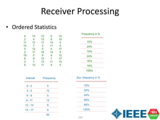
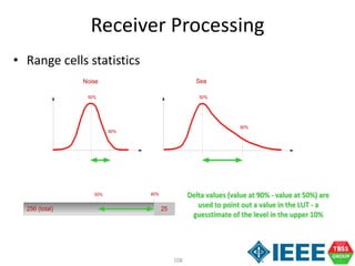
107
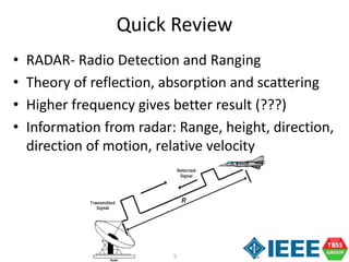
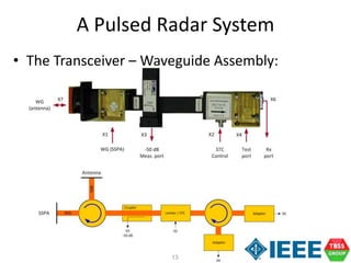
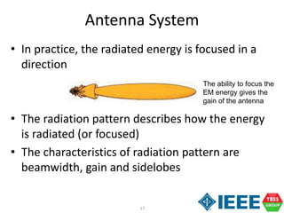
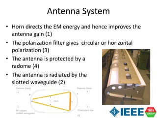
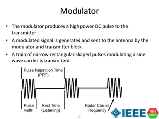
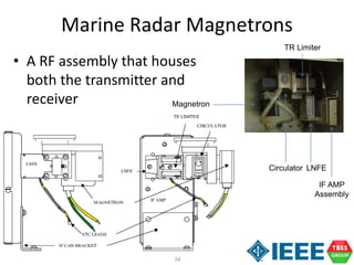
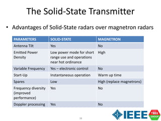
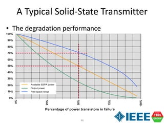
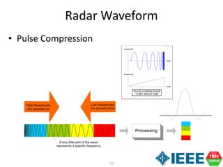
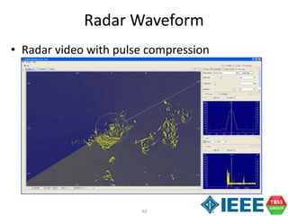
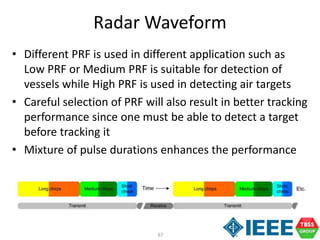
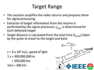
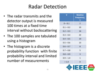
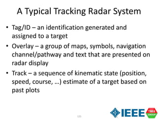
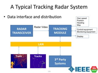
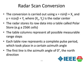
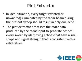
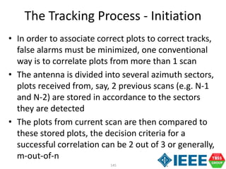
LUT
(Look-up
Table)
The difference in signal level
between 50% and 90%
fractile, is used to point out an
additional attenuation in the
LUT
- Att.
Signal Level
(90% - 50%)
Interval Frequency [%]
Frequency [%],
accumulated
0-15 8,6 8.6
16-31 11,7 20.3
32-47 18,0 38.3
48-63 11,7 50.0
64-79 1,6 51.6
80-95 5,5 57.1
96-111 4,7 61.8
112-127 4,7 66.5
128-143 5,5 72.0
144-159 3,1 75.1
160-175 3,9 79.0
176-191 5,5 84.5
192-207 3,9 88.4
208-223 3,9 92.3
224-241 3,1 95.4
240-255 4,7 100.0
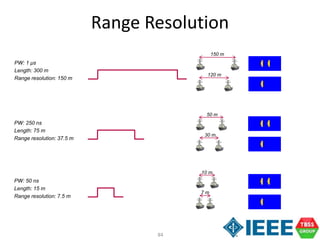
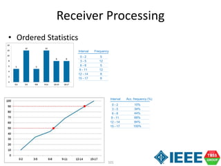
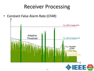
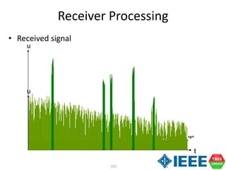
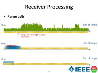
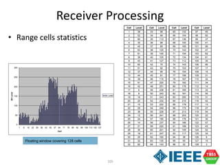
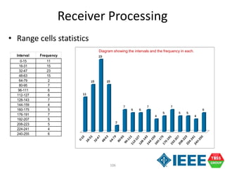
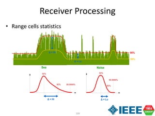
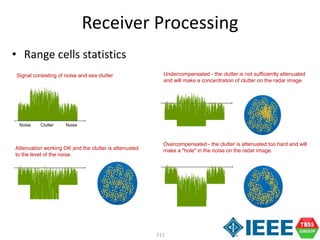
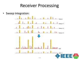
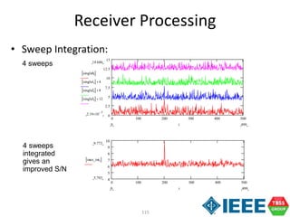
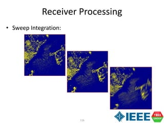
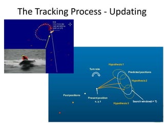
Receiver Processing

108
Noise Sea
50%
90%
50%
90%
256 (total)
50% 90%
25
Delta values (value at 90% - value at 50%) are
used to point out a value in the LUT - a
guesstimate of the level in the upper 10%
Delta values (value at 90% - value at 50%) are
used to point out a value in the LUT - a
guesstimate of the level in the upper 10%
Receiver Processing

109
90%
50%
Δ = Hi
Δ = Lo
50%
90%
Sea
Δ = Hi
99.9999%
50%
90%
Noise
Δ = Lo
99.9999%
Receiver Processing

110
50%
90%
Sea
Δ = Hi
99.9999%
50%
90%
Noise
Δ = Lo
99.9999%
Δ value
The delta value is used to guesstimate
the value at 99.9999%, PFA = 10-6
.
The value of the attenuation to obtain
this, is fetched from the LUT and
therefore the attenuation depends on
the distribution curves
Δ value
LUT
Δvalue
90%
CFAR: 10-6
Receiver Processing

111
Noise Clutter Noise
Signal consisting of noise and sea clutter
Attenuation working OK and the clutter is attenuated
to the level of the noise.
Undercompensated - the clutter is not sufficiently attenuated
and will make a concentration of clutter on the radar image.
Overcompensated - the clutter is attenuated too hard and will
make a "hole" in the noise on the radar image.
Receiver Processing

112
Page 11 of
11
Receiver Processing
• CFAR effect:

113
Average is stored in weep n+3
For the next integration cycle
sweep n+1 will be sweep n
Sweep
n+3
Sweep n+2
Sweep n+1
Sweep n
Video
Noise
Receiver Processing
• Sweep Integration:

114
Sweep n
Sweep n+1
Sweep n+2
Sweep n+3
ADD
ADD / 4
Receiver Processing

115
0 100 200 300 400 500
0
2.5
5
7.5
10
12.5
15
14.686
2.19 10
3

single0i
single1i 4
single2i 8
single3i 12
4990 i
4 sweeps
4 sweeps
integrated
gives an
improved S/N
0 100 200 300 400 500
4
5
6
7
8
9
10
9.773
5.793
inco_inti
4990 i
Receiver Processing

116
Receiver Processing

117
Receiver Processing
• Scan Correlation
– The radar performs sliding window scan-to-scan correlation
for each range-azimuth cell to provide clutter discrimination
– This is done to discriminate between clutter and targets that
are of interest to the operator

118
Scan Correlation
• One channel performs sliding window scan-to-scan correlation
over 3 consecutive scans to discriminate between clutter and
extremely small targets with speeds up to e.g. 8 knots - the actual
speed limit is determined by the antenna rotation speed, the pulse
width and the range
• A second channel performs sliding window scan-to-scan
correlation over 2 consecutive scans in order to discriminate
between clutter and small targets with speeds up to e.g. 16 knots -
the actual speed limit is also here determined by the antenna
rotation speed, the pulse width and the range
• A third channel without scan-to-scan correlation to detect targets
of medium and large size (RCS) at any speed
Receiving Processing

119
• Scan Correlation

120
Gate signal
No gate signal
AND
Gate signal
No gate signal
AND
1 3 5 7 92 4 6 8
1
0Scan n-2
1 3 5 7 92 4 6 8
1
0Scan n-1
3 s
1 3 5 7 92 4 6 8
1
0
Clutter
1 3 5 7 92 4 6 8
1
0Scan n
3 s
Target Returned echo (PW = 500 ns)
Resolution cells (10 x 7.5 m)
Threshold
Level
Target Returned echo (PW = 500 ns)
Resolution cells (10 x 7.5 m)
Threshold
Level

121
ANDAND
1 3 5 72 4 6 8Scan n-2
1 3 5 72 4 6 8Scan n-1
3 s
1 3 5 72 4 6 8Scan n
3 s
Gate signal

122
A Typical Tracking Radar System
• The receiver decides that an object has been
detected (signal strength > threshold)
• The signal processor will determine the presence of
real targets and rejects the unwanted returns

123
• The data extractor will determine the target
measurements such as range, azimuth and/or
elevation (2D or 3D)

124
• The data processor will perform the association,
tracking and prediction task and maintains the
target database
• Echo – a group of coherent detections within the
same sweep
• Plot – a group of echoes within the same radar
scan correlated in range and bearing in
accordance to some pre-defined criteria such as
center of gravity, peak amplitude, peak size, …

125
• Tag/ID – an identification generated and
assigned to a target
• Overlay – a group of maps, symbols, navigation
channel/pathway and text that are presented on
radar display
• Track – a sequence of kinematic state (position,
speed, course, …) estimate of a target based on
past plots

126
• A typical radar with
tracker is made up of
tracking
module/algorithm,
display, scan
conversion and user
interface
• The exchange of data
is achieved via a local
area network (LAN)
LAN AREA NETWORK

127
• The processors are connected to the system bus
or network where radar input signals (ACP, ARP)
and videos (targets, clutters) are processed and
shared
• The radar videos are packaged in LAN message
protocol for sharing and further processing
• The target echoes are identified as plots and
tracking process is initiated
• The tracking information is then distributed
via the LAN

128
• A typical radar data distribution over network
Video, plots,
tracks, BITE,
control
LAN
RADAR
TRANSCEIVER
AND PROCESSOR
3rd PARTY
CONTROL AND
COMMNAND
SYSTEM
RADAR DISPLAY
AND
WORKSTATION
RADAR SERVICE
TOOL

129
• Data interface and distribution
RADAR
TRANSCEIVER
TRACKING
MODULE
Radar Video
LAN
Own speed
Position
Heading
Map
Control equipment
Monitoring equipment
Display
3rd Party
Systems
TracksTrails

130
• Usually, extractor and tracker are housed under
one single module
Data
Extractor
Data Processor
(Tracker)
Plots
Settings
Radar
Video
Platform and
Navigation
Data
Map Data
Status
Tracks
Plot Position
External
Tracks

131
Radar Scan Conversion
• The radar scan
converter receives raw
radar video and
converts it into a
format for raster scan
display
• The radar interface
takes in
– video and antenna
signal from the radar
– the radar input gain
and

132
• A surveillance radar supplies its measured data in polar
coordinates, i.e. in range-azimuth format (r,b)
• Radar scan conversion involves the transformation of data in a
range-azimuth format to an x-y format for a raster-scan display

133
• The conversion is carried out using x = rsinb + Xc and
y = rcosb + Yc where (Xc, Yc) is the radar center
• The radar stores its raw data into a table called Polar
Store (e.g a 256K cells)
• The table columns represent all possible measurable
range steps
• Each table row represents a complete pulse period,
which took place in a certain azimuth angle
• The first line is the azimuth angle of 0°, the north
direction

134
• The radar interface will also accept the existing
azimuths (2048 – 11-bit antenna word) per 360
• The actual acquired data in the form of rho-theta is
stored in the display frame stores (e.g. 2048 by 2048)
• The scan conversion algorithm handles the 2048 by
2048 resolution display in real time up to 60 r.p.m.
antenna rotation rate
• The scan conversion process is controllable
• General graphics drawing capability is provided for
flight/navigational plan and mask definition

135
• Scan conversion can also be performed in several
windows
• The display controller graphics accelerator of the
display card is supported by at least 2 GB of RAM to
provide exceptional flexibility for generating
combined graphics and radar video and with an
output resolution of up to say 1600 by 1280
• The display shall consists of symbols and targets
layer, radar video layer which fades and become
transparent and maps and charts layer

136
Plot Extractor
• A radar plot is a group of connected range-azimuth
cells whose measured signal strength exceeds a
defined threshold
• A plot is displayed which the video signal strength is
larger than the threshold
• Technique such as STC (Sensitivity Time Control)
improves the target detection by suppressing the
echoes nearby the radar

137
Plot Extractor
• In ideal situation, every target (wanted or
unwanted) illuminated by the radar beam during
the present sweep should result in only one echo
• The plot extractor processes the radar data
produced by the radar input to generate echoes
every sweep by identifying echoes that have a size,
shape and signal strength that is consistent with a
valid return

138
Plot Extractor
• Plot extractor is software application that analyses radar
video and detects potential targets
• Processing is based on three main phases:
– clutter suppression
– adaptive thresholding
– plot extraction
• Clutter suppression can be based on Clutter Map Constant
False Alarm Rate (CFAR) algorithm
• Adaptive thresholding implemented can be Cell Averaging
CFAR (CA-CFAR) detection
• Plot extraction is detection of target-like shapes among
video samples that exceed the threshold using standard
m-of-n separation criterion

139
Plot Extractor
• Plot Extractor and radar input is direct (not
TCP/IP)
• Since Plot Extractor is the only component that
requires high sample rate, it is optimal to place it
on the same machine as the signal source
• Another consumer of raw video samples is Radar
Display
• Since Radar Display requires lower sample rates,
Plot Extractor also performs downsampling of
the video before streaming it on the network

140
The Tracking Process
• A tracking process is generally made up of 3
stages namely, Initiation, Updating and
Termination

141
The Tracking Process
• A good tracker will be able to provide better
detection of highly maneuvering small targets

142
The Tracking Process - Initiation
• When a target is acquired, the initiate position
(Cartesian coordinates) is taken from the tracker
ball (some call it order marker) or generated by
processor
• The radar return
defined by range
and bearing
(polar
coordinates)

143
• The conversion from polar to Cartesian
coordinates is carried out every antenna scan,
when a track is confirmed, the target speed and
course can be calculated by the data processor

144
• The initiation process
Predicted position
Track
Radial acceleration
Tangential acceleration
Minimum speed
Maximum speed

145
• In order to associate correct plots to correct tracks,
false alarms must be minimized, one conventional
way is to correlate plots from more than 1 scan
• The antenna is divided into several azimuth sectors,
plots received from, say, 2 previous scans (e.g. N-1
and N-2) are stored in accordance to the sectors
they are detected
• The plots from current scan are then compared to
these stored plots, the decision criteria for a
successful correlation can be 2 out of 3 or generally,
m-out-of-n

146
• Consider a plot PN in sector S of antenna scan N,
an initiation window will be opened at this plot
position, a search is then made in N-1 plot
database to find a plot within this window

147
• Assuming only plots in sectors S-1, S and S+1 are
search (for minimized comparison time) and that
a plot PN-1 is found, then another search is
carried out in N-2 plot database

148
• If the search is successful in N-2 plot database then the
primary track initiation is successful, however, if there is no
plot in N-2 plot database, then the primary track initiation
can also be considered successful if the decision criteria is 3-
out-of-2

149
• The available plots are then used to calculate the target
position in x-y coordinates, the speed vector and the
predicted next position (by filtering)
• They are also used to determine the quality of the track
(centroid) and subsequently the gate size
Centroid is of a target
is defined as the
value of independent
variable (in time)
where the area under
the target spectrum to
the right equals to the
left

150
• Given a plot at radar scan
N, it is necessary to
determine the shade
(usually not
implemented) and size of
the correlation gate in
order to capture the plot
at scan N+1, the gate is
usually defined in terms
of range and azimuth

151
• The prediction process
With good
predictions
the search
window
gets smaller
With bad
predictions
the search
window
gets bigger

152
• Correlation window eliminates the unlikely plot-to-
track pairings and hence reduce unnecessary
computation
• During the initial acquisition, usually the 1st 2 scans,
the processor does not have sufficient knowledge of
the target’s course and speed, the gate is larger to
increase the match probability
• After several scans, the target’s motion is better
known, the gate size reduces, the gate size is
determined by the radar measurement error and
possible maneuvering

153
• After the new track is initiated and vector
generated, track updating is necessary to update the
track with correct plots obtained so as to update
current track information (position, speed, course)
and predict future position
• The 1st task involves comparing the incoming plots
with known tracks to obtain a list of all possible
plot-track pairs
• One commonly used comparison method which
results shortest possible comparison time is to
organized the tracks such that they are compared
with smallest possible no. of plots
The Tracking Process - Updating

154
• Depending on implementations, a central sector
covering >1 track sectors, e.g. 2 track sectors and
therefore 3 plot sectors, is defined for detecting
plots that have evolved to non-adjacent sectors
(fast moving targets or small sector size)
• If there exists a central sector, an unsuccessful
correlation of plots (from the 2 adjacent plots) to
a track, comparison is made with plots in the
central sector

155
• 1 simple way to resolve such problem is to
generate a plot-track distance matrix, a plot is
then associated to a track it lies within the gate,
the distance between the correlated plot and the
track is computed and stored in the matrix
• After the comparison cycle, some common
situations can occur
– 1 plot is associated to 1 track
– 1 plot is associated to several tracks
– several plots are assigned to 1 track
– no associated of plot to any track

156
• Consider a plot-track distance matrix, it is
obvious that plot 3 is associated to track 3
(deleted from matrix), plot 1 is associated to
track 1 (delete from matrix)
Track 1 Track 2 Track 3
Plot 1 1 4 15
Plot 2 3 3 13
Plot 3 12 10 3
Plot 4 5 3 10

157
• Plot 2 and 4 can be associated to track 2, one
simple way to resolve the problem is to assign
plot 2 randomly (wrong assignment will be
rectified after a few more scans)
• The remaining plots are considered for new track
initiation and remaining tracks can considered
termination
Track 1 Track 2 Track 3
Plot 1 1 4 15
Plot 2 3 3 13
Plot 3 12 10 3
Plot 4 5 3 10

158
• After association, the track information are
stored in the target database; the measured
position (if there is an associated plot) is
updated, otherwise the predicted position is
used
• Predicted position is obtained by filtering (e.g.
Kalman or ab filter) which filters and predicts
target position

159
Predicted position
Track
Updated track
Out of search window
Out of shape
New search window
New prediction
• The plot-to-track correlation

160
• The quality factor, status of the track, gate size
and position is computed
• The quality factor of a track depends on the
track history (how good it was), it is used to
compute the gate size for the next scan (smaller
or larger)
• The quality factor is computed as
where K = +ve when there is a plot in the gate
and K = -ve there is no plot in the gate
KQQ nn 1

161

162
• This process is performed once every scan for
every track, an associated plot is known as a hit
where a non-associated plot is a miss
• A track is cancelled automatically when plot is
absent for a predefined no. of scans consecutive
or Q = 0 (no point tracking)
• A track is also terminated manually when drop
track function is invoked
• This erases all data corresponding to the track in
the target table, the lost target symbol is
displayed for reference
The Tracking Process - Termination

163
• A miss
The Tracking Process - Termination
Predicted position
Track
This will count as a lack –
no update found

A Tutorial on Radar System Engineering

Recommended

Recommended

More Related Content

What's hot

What's hot (20)

Similar to A Tutorial on Radar System Engineering

Similar to A Tutorial on Radar System Engineering (20)

More from TBSS Group

More from TBSS Group (20)

Recently uploaded

Recently uploaded (20)

A Tutorial on Radar System Engineering