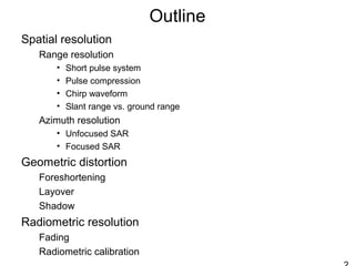
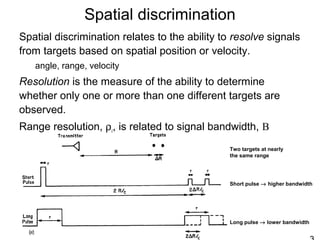
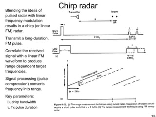
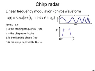
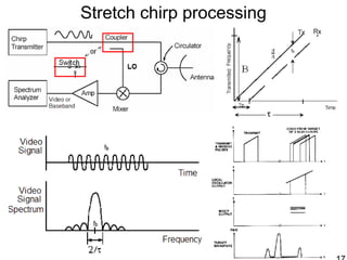
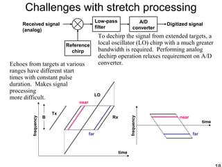
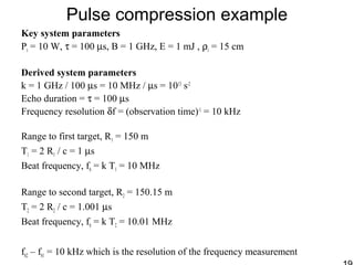
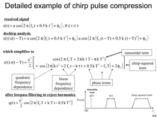
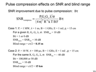
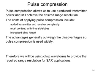
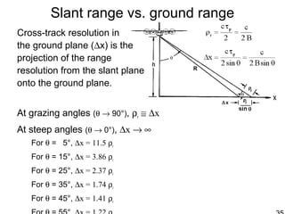
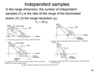
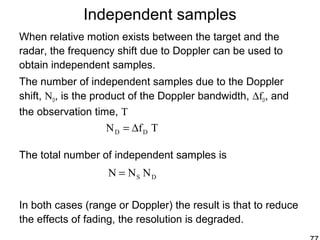
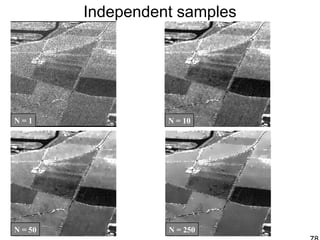
This document discusses synthetic aperture radar (SAR) and pulse compression techniques. It explains that pulse compression allows radar systems to achieve fine range resolution using long duration, low power pulses by modulating the pulses with linear frequency modulation (chirp) and then correlating the received signal with a reference chirp. This improves the signal to noise ratio compared to using short pulses directly. The document covers topics such as range resolution, pulse compression, chirp waveforms, stretch processing, correlation processing, window functions, and how pulse compression affects signal to noise ratio and blind range.
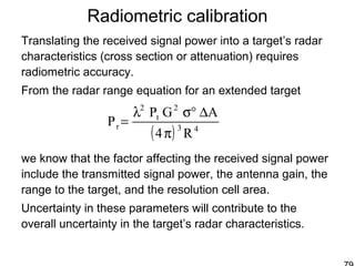
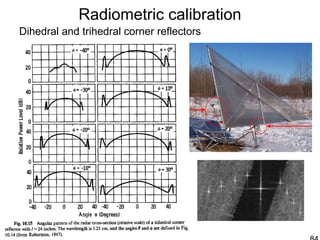
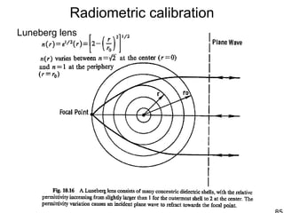
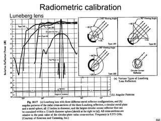
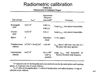
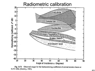
![Radiometric calibration
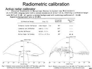
Active radar calibrator [Brunfeldt and Ulaby, IEEE Trans. Geosci. Rem. Sens., 22(2),
pp. 165-169, 1984.]](https://image.slidesharecdn.com/826sarbasics-s09-150331131813-conversion-gate01/85/synthetic-aperture-radar-88-320.jpg)