Downloaded 741 times

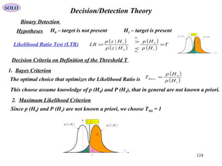
![4
SOLO
The transmitted RADAR RF
Signal is:
( ) ( ) ( )[ ]ttftEtEt 0000 2cos ϕπ +=
E0 – amplitude of the signal
f0 – RF frequency of the signal
φ0 –phase of the signal (possible modulated)
The returned signal is delayed by the time that takes to signal to reach the target and to
return back to the receiver. Since the electromagnetic waves travel with the speed of light
c (much greater then RADAR and
Target velocities), the received signal
is delayed by
c
RR
td
21 +
≅
The received signal is: ( ) ( ) ( ) ( )[ ] ( )tnoisettttfttEtE dddr +−+−⋅−= ϕπα 00 2cos
To retrieve the range (and range-rate) information from the received signal the
transmitted signal must be modulated in Amplitude or/and Frequency or/and Phase.
ά < 1 represents the attenuation of the signal
RADAR Signal Processing
RADAR Signals](https://image.slidesharecdn.com/1-radarsignalprocessing-150117083950-conversion-gate01/85/1-radar-signal-processing-4-320.jpg)
![5
SOLO
The received signal is:
( ) ( ) ( ) ( )[ ] ( )tnoisettttfttEtE dddr +−+−⋅−= ϕπα 00 2cos
( ) ( ) tRRtRtRRtR ⋅+=⋅+= 222111 &
We want to compute the delay time td due to the time td1 it takes the EM-wave to reach
the target at a distance R1 (at t=0), from the transmitter, and to the time td2 it takes the
EM-wave to return to the receiver, at a distance R2 (at t=0) from the target. 21 ddd ttt +=
According to the Special Theory of Relativity
the EM wave will travel with a constant
velocity c (independent of the relative
velocities ).21 & RR
The EM wave that reached the target at
time t was send at td1 ,therefore
( ) ( ) 111111 ddd tcttRRttR ⋅=−⋅+=− ( )
1
11
1
Rc
tRR
ttd
+
⋅+
=
In the same way the EM wave received from the target at time t was reflected at td2 ,
therefore
( ) ( ) 222222 ddd tcttRRttR ⋅=−⋅+=− ( )
2
22
2
Rc
tRR
ttd
+
⋅+
=
RADAR Signal Processing](https://image.slidesharecdn.com/1-radarsignalprocessing-150117083950-conversion-gate01/85/1-radar-signal-processing-5-320.jpg)
![6
SOLO
The received signal is:
( ) ( ) ( ) ( )[ ] ( )tnoisettttfttEtE dddr +−+−⋅−= ϕπα 00 2cos
21 ddd ttt += ( )
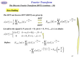
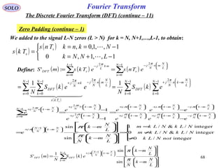
1
11
1
Rc
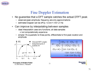
tRR
ttd
+
⋅+
= ( )
2
22
2
Rc
tRR
ttd
+
⋅+
=
( ) ( )
2
22
1
11
21
Rc
tRR
Rc
tRR
tttttttt ddd
+
⋅+
−
+
⋅+
−=−−=−
+
−
+
−
+
+
−
+
−
=−
2
2
2
2
1
1
1
1
2
1
2
1
Rc
R
t
Rc
Rc
Rc
R
t
Rc
Rc
tt d
From which:
or:
Since in most applications we can
approximate where they appear in the arguments of E0 (t-td), φ (t-td),
however, because f0 is of order of 109
Hz=1 GHz, in radar applications, we must use:
cRR <<21,
1,
2
2
1
1
≈
+
−
+
−
Rc
Rc
Rc
Rc
( )
−⋅
++
−⋅
+=
−⋅
−+
−⋅
−⋅≈− 2
.
201
.
10
22
0
11
00
2
1
2
1
2
12
1
2
12
1
21
D
Ralong
FreqDoppler
DD
Ralong
FreqDoppler
Dd ttffttff
c
R
t
c
R
f
c
R
t
c
R
fttf
( ) ( ) ( ) ( ) ( )[ ] ( )tnoisettttffttEtE ddDdr +−+−⋅+−= ˆˆˆ2cosˆ 00 ϕπα
where 21
2
2
1
121
2
02
1
01
ˆˆˆ,,,ˆˆˆ,
2ˆ,
2ˆ
dddddDDDDD ttt
c
R
t
c
R
tfff
c
R
ff
c
R
ff +=≈≈+=−≈−≈
Finally
RADAR Signal Processing
Doppler Effect](https://image.slidesharecdn.com/1-radarsignalprocessing-150117083950-conversion-gate01/85/1-radar-signal-processing-6-320.jpg)
![7
SOLO
The received signal model:
( ) ( ) ( ) ( ) ( )[ ] ( )tnoisettttffttEtE ddDdr +−+−⋅+−≈ ϕπα 00 2cos
Delayed by two-
way trip time
Scaled down
Amplitude Possible phase
modulated
Corrupted
By noise
Doppler
effect
We want to estimate:
• delay td range c td/2
• amplitude reduction α
• Doppler frequency fD
• noise power n (relative to signal power)
• phase modulation φ
Return to Table of Content](https://image.slidesharecdn.com/1-radarsignalprocessing-150117083950-conversion-gate01/85/1-radar-signal-processing-7-320.jpg)
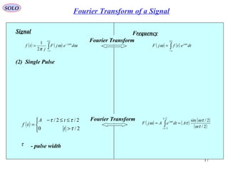
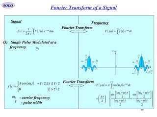
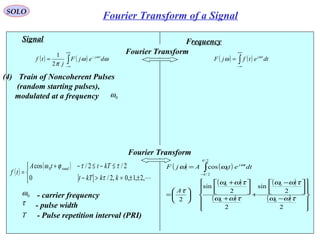
![9
SOLO
( )tf
2
τ
2
τ
−
A
∞→t
2
τ
+T
2
τ
−T
A
2
τ
+−T
2
τ
−−T
A
t←∞−
T T
NONCOHERENT PULSESCOHERENT PULSES
( )tf
t
A
2
τ
2
τ
−T
AA
T T
A
2
2
τ
+T
2
2
τ
−T
A
T T
A
2
τ
− 2
τ
+T
TN
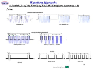
PULSED (UNCODED)
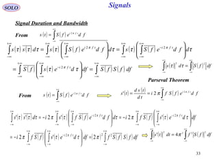
A Partial List of the Family of RADAR Waveforms
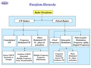
PRI – Pulse Repetition Interval PRF – Pulse Repetition Frequency
τ – Pulse Width [μsec]
PRF = 1/PRI
Pulse Duty Cycle = DC = τ / PRI = τ * PRF
Paverrage = DC * Ppeak
Pulse Waveform Parameters
Continuous Waves (CW)
Pulses
• Coherent – Phase is predictable from pulse-to-pulse
• Non-coherent – Phase from pulse-to-pulse is not predictable
Waveform Hierarchy](https://image.slidesharecdn.com/1-radarsignalprocessing-150117083950-conversion-gate01/85/1-radar-signal-processing-9-320.jpg)
![12
SOLO
Radar Generic Procedures:
Matched Filters in RADAR Systems
• Transmits high frequency (f0) EM signal: ( ) ( ) ( )[ ]ttftEtEt 0000 2cos ϕπ +=
( ) ( ) ( ) ( ) ( )[ ] ( )tnoisettttffttEtE ddDdr +−+−⋅+−≈ ϕπα 00 2cos
• Receives low power reflected EM signal that contains doppler information (f0 + fD):
• Down-converts to Intermediate Frequency (IF) signal (fIF + fD), Amplifies at Low Noise,
and Automatically Controls the Gain (AGC) of the receiver:
( ) ( ) ( ) ( ) ( )[ ] ( )tnoisettttffttEGtE IFddDIFdIFIF +−+−⋅+−≈ ϕπα 2cos0
• Down-converts to Video Frequency (V) signal (fV + fD), (often using a Synchronous I,Q
configuration), samples the video (A/D) for Digital Signal Processing.
• The Digital Signal Processing (DSP) performs Fast Fourier Transforms (FFT),
to produce the Data Cube (Range, Doppler, Receiving Channels). Using the data
DSP detects the potential targets, and computes the receiving delay td (Range),
Doppler frequency (closing velocity), angular target position. According to the
Radar policy, he will acquire the targets of interest, and will track them.
Doing this he prevents unwanted signal (Clutter, ECM, …) to interfere with
the target of interest received signals.
This presentation deals with some aspects of the Radar Digital Processing.](https://image.slidesharecdn.com/1-radarsignalprocessing-150117083950-conversion-gate01/85/1-radar-signal-processing-12-320.jpg)
![14
Fourier Transform
( ) ( ){ } ( ) ( )∫
+∞
∞−
−== dttjtftfF ωω exp:F
SOLO
Jean Baptiste Joseph
Fourier
1768-1830
F (ω) is known as Fourier Integral or Fourier Transform
and is in general complex
( ) ( ) ( ) ( ) ( )[ ]ωφωωωω jAFjFF expImRe =+=
Using the identities
( ) ( )t
d
tj δ
π
ω
ω =∫
+∞
∞− 2
exp
we can find the Inverse Fourier Transform ( ) ( ){ }ωFtf -1
F=
( ) ( ) ( ) ( ) ( )
( ) ( )( ) ( ) ( ) ( ) ( )[ ]00
2
1
2
exp
2
expexp
2
exp
++−=−=−=
−=
∫∫ ∫
∫ ∫∫
∞+
∞−
∞+
∞−
∞+
∞−
+∞
∞−
+∞
∞−
+∞
∞−
tftfdtfd
d
tjf
d
tjdjf
d
tjF
ττδττ
π
ω
τωτ
π
ω
ωττωτ
π
ω
ωω
( ) ( ){ } ( ) ( )∫
+∞
∞−
==
π
ω
ωωω
2
exp:
d
tjFFtf -1
F
( ) ( ) ( ) ( )[ ]00
2
1
++−=−∫
+∞
∞−
tftfdtf ττδτ
If f (t) is continuous at t, i.e. f (t-0) = f (t+0)
This is true if (sufficient not necessary)
f (t) and f ’ (t) are piecewise continue in every finite interval1
2 and converge, i.e. f (t) is absolute integrable in (-∞,∞)( )∫
+∞
∞−
dttf](https://image.slidesharecdn.com/1-radarsignalprocessing-150117083950-conversion-gate01/85/1-radar-signal-processing-14-320.jpg)
![15
( )atf −
-1
F
F ( ) ( )ωω ajF −exp
Fourier TransformSOLO
( )tf
-1
F
F
( )ωFProperties of Fourier Transform (Summary)
Linearity1
( ) ( ){ } ( ) ( )[ ] ( ) ( ) ( )ωαωαωαααα 221122112211 exp: FFdttjtftftftf +=−+=+ ∫
+∞
∞−
F
Symmetry2
( )tF
-1
F
F
( )ωπ −f2
Conjugate Functions3 ( )tf *
-1
F
F
( )ω−*
F
Scaling4 ( )taf
-1
F
F
a
F
a
ω1
Derivatives5 ( ) ( )tftj
n
−
-1
F
F ( )ω
ω
F
d
d
n
n
( )tf
td
d
n
n
-1
F
F
( ) ( )ωω Fj
n
Convolution6
( ) ( )tftf 21
-1
F
F ( ) ( )ωω 21
* FF( ) ( ) ( ) ( )∫
+∞
∞−
−= τττ dtfftftf 2121
:*
-1
F
F ( ) ( )ωω 21
FF
( ) ( ) ( ) ( )∫∫
+∞
∞−
+∞
∞−
= ωωω
π
dFFdttftf 2
*
12
*
1
2
1
Parseval’s Formula7
Shifting: for any a real8
( ) ( )tajtf exp
-1
F
F ( )aF −ω
Modulation9 ( ) ttf 0
cos ω -1
F
F
( ) ( )[ ]00
2
1
ωωωω −++ FF
( ) ( ) ( ) ( ) ( ) ( )∫∫∫
+∞
∞−
+∞
∞−
+∞
∞−
−=−= ωωω
π
ωωω
π
dFFdFFdttftf 212121
2
1
2
1](https://image.slidesharecdn.com/1-radarsignalprocessing-150117083950-conversion-gate01/85/1-radar-signal-processing-15-320.jpg)
![20
( ) ( )∫
+∞
∞−
−
= ωω
π
ω
dejF
j
tf tj
2
1
Signal
( )
( )
( ) ( )( ) ( )( )[ ]
−++
+=
±±=>−
≤−≤−
=
∑
∞
=1
000
0
coscos
2
2
sin
cos
,2,1,0,2/0
2/2/cos
n
PRPR
PR
PR
series
Fourier
tntn
n
n
t
T
A
kkkTt
kTttA
tf
ωωωω
τω
τω
ω
τ
τ
ττω
τ - pulse width
Frequency
( ) ( )∫
+∞
∞−
= dtetfjF tjω
ω
Fourier Transform
Fourier Transform
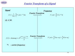
0ω - carrier frequency
5) Train of Coherent Pulses,
of infinite length,
modulated at a frequency 0ω
T - Pulse repetition interval (PRI)
( ) ( ) ( ){
( ) ( ) ( ) ( )[ ]
+−+−+−−++
+
−+=
∑
∞
=1
0000
00
2
2
sin
2
n
PRPRPRPR
PR
PR
nnnn
n
n
T
A
jF
ωωδωωδωωδωωδ
τω
τω
ωδωδ
τ
ω
T/1 - Pulse repetition frequency (PRF)
TPR /2πω =
SOLO
Fourier Transform of a Signal](https://image.slidesharecdn.com/1-radarsignalprocessing-150117083950-conversion-gate01/85/1-radar-signal-processing-20-320.jpg)
![21
( ) ( )∫
+∞
∞−
−
= ωω
π
ω
dejF
j
tf tj
2
1
Signal
( )
( )
( ) ( )( ) ( )( )[ ]
−++
+=
±±=>−
≤−≤−
=
∑
∞
=
≤≤−
1
000
22
0
coscos
2
2
sin
cos
2/,,2,1,0,2/0
2/2/cos
n
PRPR
PR
PRNT
t
NT
tntn
n
n
t
T
A
NkkkTt
kTttA
tf
ωωωω
τω
τω
ω
τ
τ
ττω
τ - pulse width
Frequency
( ) ( )∫
+∞
∞−
= dtetfjF tjω
ω
Fourier Transform
Fourier Transform
0ω - carrier frequency
6) Train of Coherent Pulses,
of finite length N T,
modulated at a frequency 0ω
T - Pulse repetition interval (PRI)
( )
( )
( )
( )
( )
( )
( )
( )
( )
( )
( )
( )
( )
−−
−−
+
+−
+−
+
+
+
+
−+
−+
+
++
++
+
+
+
=
∑
∑
∞
=
∞
=
1
0
0
0
0
0
0
1
0
0
0
0
0
0
2
2
sin
2
2
sin
2
2
sin
2
2
sin
2
2
sin
2
2
sin
2
2
sin
2
2
sin
2
n
PR
PR
PR
PR
PR
PR
n
PR
PR
PR
PR
PR
PR
TN
n
TN
n
TN
n
TN
n
n
n
TN
TN
TN
n
TN
n
TN
n
TN
n
n
n
TN
TN
T
A
jF
ωωω
ωωω
ωωω
ωωω
τω
τω
ωω
ωω
ωωω
ωωω
ωωω
ωωω
τω
τω
ωω
ωω
τ
ω
T/1 - Pulse repetition frequency (PRF)
TPR /2πω =
SOLO
Fourier Transform of a Signal](https://image.slidesharecdn.com/1-radarsignalprocessing-150117083950-conversion-gate01/85/1-radar-signal-processing-21-320.jpg)
![22
Signal
( ) ( )
+=
±±=>−
≤−≤−
= ∑
∞
=1
1 cos
2
2
sin
21
,2,1,0,2/0
2/2/
n
PR
PR
PR
Series
Fourier
tn
n
n
T
A
kkkTt
kTtA
tf ω
τω
τω
τ
τ
ττ
τ - pulse width
0ω - carrier frequency
6) Train of Coherent Pulses,
of finite length N T,
modulated at a frequency 0ω
T - Pulse repetition interval (PRI)
T/1 - Pulse repetition frequency (PRF)
TPR /2πω =
( ) ( )tAtf 03 cos ω=
t
A A
( )tf1
t
2
τ
2
τ
−T
A
T T
2
2
τ+T
2
2
τ−T
T T
2
τ− 2
τ+T
( )tf2
t
TN
2/TN2/TN−
( ) ( ) ( ) ( )tftftftf 321 ⋅⋅=
( ) ( ) ( ) ( )
( )
( ) ( )( ) ( )( )[ ]
−++
+=
±±=>−
≤−≤−
=⋅⋅=
∑
∞
=
≤≤−
1
000
22
0
321
coscos
2
2
sin
cos
2/,,2,1,0,2/0
2/2/cos
n
PRPR
PR
PRNT
t
NT
tntn
n
n
t
T
A
NkkkTt
kTttA
tftftftf
ωωωω
τω
τω
ω
τ
τ
ττω
( )
>
≤≤−
=
2/0
2/2/1
2
TNt
TNtTN
tf ( ) ( )ttf 03 cos ω=
SOLO
Fourier Transform of a Signal](https://image.slidesharecdn.com/1-radarsignalprocessing-150117083950-conversion-gate01/85/1-radar-signal-processing-22-320.jpg)
![25
RADAR SignalsSOLO
Waveforms
( ) ( ) ( )[ ]tttats θω += 0cos
a (t) – nonnegative function that represents any amplitude modulation (AM)
θ (t) – phase angle associated with any frequency modulation (FM)
ω0 – nominal carrier angular frequency ω0 = 2 π f0
f0 – nominal carrier frequency
Transmitted Signal
( ) ( ) ( )[ ]{ }ttjtats θω += 0exp
Phasor (complex) Transmitted Signal
Return to Table of Content](https://image.slidesharecdn.com/1-radarsignalprocessing-150117083950-conversion-gate01/85/1-radar-signal-processing-25-320.jpg)
![26
RADAR SignalsSOLO
Quadrature Form
( ) ( ) ( )[ ]
( ) ( )[ ] ( ) ( ) ( )[ ] ( )tttattta
tttats
00
0
sinsincoscos
cos
ωθωθ
θω
−=
+=
where: ( ) ( ) ( )[ ]
( ) ( ) ( )[ ]ttats
ttats
Q
I
θ
θ
sin
cos
=
=
( ) ( ) ( ) ( ) ( )ttsttsts QI 00 sincos ωω −=
One other form: ( ) ( ) ( )[ ] ( ) ( ) ( )
[ ]tjtjtjtj
ee
ta
tttats θωθω
θω −−+
+=+= 00
2
cos 0
( ) ( ) ( )[ ]tjtj
etgetgts 00 *
2
1 ωω −
+= ( ) ( ) ( ) ( ) ( )tj
QI etatsjtstg θ
=+=:
Envelope of the signal
( ) ( ) tj
etgts 0ω
=
Phasor (complex) Transmitted Signal
Transmitted Signal
Return to Table of Content](https://image.slidesharecdn.com/1-radarsignalprocessing-150117083950-conversion-gate01/85/1-radar-signal-processing-26-320.jpg)
![27
RADAR SignalsSOLO
Spectrum
Define the Fourier Transfer F
( ) ( ){ } ( ) ( )∫
+∞
∞−
−== dttjtstsS ωω exp:F ( ) ( ){ } ( ) ( )∫
+∞
∞−
==
π
ω
ωωω
2
exp:
d
tjSSts 1-
F
( ) ( ) ( )[ ]tjtj
etgetgts 00 *
2
1 ωω −
+= ( ) ( ) ( )[ ]0
*
0
2
1
ωωωωω −−+−= GGS-1
F
F
-1
F
F
( ) ( ) ( ) ( ) ( )tj
QI etatsjtstg θ
=+=:
( ) ( ) ( )[ ]tttats θω += 0cos
Inverse Fourier Transfer F -1
Envelope of the signalWe defined:
Return to Table of Content](https://image.slidesharecdn.com/1-radarsignalprocessing-150117083950-conversion-gate01/85/1-radar-signal-processing-27-320.jpg)
![28
RADAR SignalsSOLO
Energy ( ) ( ) ( )[ ]tttats θω += 0cos
( ) ( ) ( )[ ]{ } ( )∫∫∫
+∞
∞−
+∞
∞−
+∞
∞−
≈++== dttadttttadttsEs
2
0
22
2
1
22cos1
2
1
: θω
Parseval’s Formula
Proof:
( ) ( ) ( ) ( )∫∫
+∞
∞−
+∞
∞−
= ωωω
π
dFFdttftf 2
*
12
*
1
2
1
( ) ( ) ( )∫
+∞
∞−
−= dttjtfF ωω exp11
( ) ( ) ( ) ( ) ( ) ( ) ( ) ( ) ( ) ( )∫∫ ∫∫ ∫∫
+∞
∞−
+∞
∞−
+∞
∞−
+∞
∞−
+∞
∞−
+∞
∞−
=−=−=
π
ω
ωω
π
ω
ωω
π
ω
ωω
22
exp
2
exp 2
*
112
*
2
*
12
*
1
d
FF
d
dttjtfFdt
d
tjFtfdttftf
( ) ( ) ( )∫
+∞
∞−
−=
π
ω
ωω
2
exp
*
2
*
2
d
tjFtf
If s (t) is real, than s (t) = s*(t) and
( ) ( ) ( )∫∫∫
+∞
∞−
+∞
∞−
+∞
∞−
=== ωω
π
dSdttsdttsEs
222
2
1
:](https://image.slidesharecdn.com/1-radarsignalprocessing-150117083950-conversion-gate01/85/1-radar-signal-processing-28-320.jpg)
![29
RADAR SignalsSOLO
Energy (continue – 1) ( ) ( ) ( )[ ]tttats θω += 0cos
( ) ( ) ( )∫∫∫
+∞
∞−
+∞
∞−
+∞
∞−
=== ωω
π
dSdttsdttsEs
222
2
1
:
( ) ( ) ( ) ( )[ ] ( ) ( )[ ]
( ) ( ) ( ) ( )
( ) ( ) ( ) ( )
−−−+−−−+
−−−−+−−
=
−−+−−−+−=
−
−−
00
0000
0
*
0
*2
00
0
*
00
*
0
00
*
0
*
0
*
4
1
4
1
ϕϕ
ϕϕϕϕ
ωωωωωωωω
ωωωωωωωω
ωωωωωωωωωω
jj
jjjj
eGGeGG
GGGG
eGeGeGeGSS
For finite band (W << ω0 ) signals (see Figure)
( ) ( ) ( ) ( )
( ) ( ) ( ) ( ) ( ) ( )∫∫∫
∫∫
∞+
∞−
∞+
∞−
∞+
∞−
+∞
∞−
−
+∞
∞−
=−−−−=−−
≈−−−=−−−
ωωωωωωωωωωωωω
ωωωωωωωωωω ϕϕ
dGGdGGdGG
deGGdeGG jj
*
0
*
00
*
0
2
0
*
0
*2
00 000
( ) ( ) gs EdGdSE
2
1
2
1
2
1
2
1
:
22
=≈= ∫∫
+∞
∞−
+∞
∞−
ωω
π
ωω
π
Return to Table of Content](https://image.slidesharecdn.com/1-radarsignalprocessing-150117083950-conversion-gate01/85/1-radar-signal-processing-29-320.jpg)
![30
RADAR SignalsSOLO
Complex and Analytic Signals
( ) ( ) ( )[ ]tttats θω += 0cos
We have the following definitions:
Real signal
( ) ( ) ( )[ ]tjtj
etgetgts 00 *
2
1 ωω −
+=
( ) ( ) ( ) ( ) ( )tj
QI etatsjtstg θ
=+=: Envelope of the signal
( ) ( ) ( )[ ] ( ) tj
etgtjtjtats 0
0exp: ω
θω =+= Complex Signal
( ) ( ) ( )[ ]tjtj
etgetgts 00 *
2
1 ωω −
+= ( ) ( ) ( )[ ]0
*
0
2
1
ωωωωω −−+−= GGS-1
F
F
( ) ( ){ } ( ){ } ( )0
0
ωωω ω
−=== GetgtsS tj
FF
( ) ( )
( )
( ) ( )ωω
ω
ωω
ωωω SU
S
GS 2
00
02
0 =
<
>
≈−=
For Band limited signals](https://image.slidesharecdn.com/1-radarsignalprocessing-150117083950-conversion-gate01/85/1-radar-signal-processing-30-320.jpg)
![31
RADAR SignalsSOLO
Complex and Analytic Signals (continue – 1)
( ) ( ) ( )[ ] ( ) tj
etgtjtjtats 0
0exp: ω
θω =+=
Complex Signal
( ) ( ){ } ( ){ } ( )0
0
ωωω ω
−=== GetgtsS tj
FF
( ) ( )
( )
( ) ( )ωω
ω
ωω
ωωω SU
S
GS 2
00
02
0 =
<
>
≈−=
For Band limited signals
Analytic Signal
The Analytic Signal is a Complex Signal chosen that its spectrum if forced to be zero for ω<0.
( ) ( ) ( ) ( )[ ] ( )ωωωωω SsignSUS +== 12:
~
( )
<−
=
>+
=
01
00
01
:
ω
ω
ω
ωsign
( )[ ] ( )[ ] ( )
t
j
tsignU
π
δωω +=+= −−
12 11
FF
The time function corresponding to the product of the spectrums of two time functions is
given by the time convolution of the two functions
( ) ( )[ ] ( ) ( )[ ] ( ) ( )
( )
( ) ( )
∫∫
+∞
∞−
+∞
∞−
−−
−
+=
−
+−=== ξ
ξ
ξ
π
ξ
ξπ
ξδξωωω d
t
sj
tsd
t
j
tsSUS 2
~~ 11
FFts](https://image.slidesharecdn.com/1-radarsignalprocessing-150117083950-conversion-gate01/85/1-radar-signal-processing-31-320.jpg)
![32
RADAR SignalsSOLO
Analytic Signal
The Analytic Signal is a Complex Signal chosen that its spectrum if forced to be zero for ω<0.
( ) ( )[ ] ( ) ( )[ ] ( ) ( )
( )
( ) ( )
∫∫
+∞
∞−
+∞
∞−
−−
−
+=
−
+−=== ξ
ξ
ξ
π
ξ
ξπ
ξδξωωω d
t
sj
tsd
t
j
tsSUS 2
~~ 11
FFts
( ) ( ) ( ) ( ) ( )tsjtsd
t
sj
ts ˆ~ +=
−
+= ∫
+∞
∞−
ξ
ξ
ξ
π
ts
or
Complex and Analytic Signals (continue – 2)
From ( ) ( )[ ] ( ) ( ) ( )ωωωωω SjSSsignS ˆ1:
~
+=+=
we have
( ) ( ) ( )
( )
( )
<+
=
>−
=−=
0
00
0
ˆ
ωω
ω
ωω
ωωω
Sj
Sj
SsignjS
Assuming a Band Limited signal we can assume that
( ) ( ) ( ) ( ) ( ) ( ) ( ) ( )tsjtststsSUSS ˆ~2
~
+=≈⇒=≈ ωωωω
where is the Hilbert Transform of s (t)( ) ( )
∫
+∞
∞−
−
= ξ
ξ
ξ
π
d
t
s
ts
1
:ˆ
(see “Hilbert Transformation” Presentation)
Return to Table of Content](https://image.slidesharecdn.com/1-radarsignalprocessing-150117083950-conversion-gate01/85/1-radar-signal-processing-32-320.jpg)
![39
( ) ( ) ( )[ ]tttats θω += 0cos
SOLO
Complex Representation of Bandpass Signals
The majority of radar signals are narrow band signals, whose Fourier transform is
limited to an angular-frequency bandwidth of W centered about a carrier angular
frequency of ±ω0.
Another form of s (t) is
( ) ( ) ( )
( )
( ) ( ) ( )
( )
( )
( ) ( ) ( ) ( )ttstts
tttatttats
QI
tsts QI
00
00
sincos
sinsincoscos
ωω
ωθωθ
−=
−=
sI (t) – in phase component sQ (t) – quadrature component
1
2
Define the signal complex envelope: ( ) ( ) ( ) ( ) ( ) ( )[ ]
( ) ( )[ ]tjta
tjttatsjtstg QI
θ
θθ
exp
sincos:
=
+=+=
Therefore:
( ) ( ) ( )[ ] ( )[ ]tstjtgts ReexpRe 0 == ω
( ) ( ) ( ) ( ) ( ) ( ) ( )tststjtgtjtgts *
2
1
2
1
exp
2
1
exp
2
1
00 +=−+= ∗
ωω
or:
3
4
( ) ( ) ( )[ ]tjtjtats θω += 0exp
Analytic (complex) signal
Return to Table of Content](https://image.slidesharecdn.com/1-radarsignalprocessing-150117083950-conversion-gate01/85/1-radar-signal-processing-39-320.jpg)
![40
( ) ( ) ( )[ ]tttats θω += 0cos
SOLO
Autocorrelation
The Autocorrelation Function is extensively used in Radar Signal Processing
( ) ( ) ( )∫
+∞
∞−
−= tdtstsRss ττ :
Real signalFor
The Autocorrelation Function is defined as:
Properties of the Autocorrelation Function:
2 ( ) ( )ττ ssss RR =−
( ) ( ) ( ) ( ) ( ) ( )ττττ
τ
ss
tt
ss RtdtststdtstsR =−=+=− ∫∫
+∞
∞−
+=+∞
∞−
'''
'
1 ( ) ( ) ( ) ( ) ( ) sss EfdfSfStdtstsR === ∫∫
+∞
∞−
+∞
∞−
*0 Es – signal energy
3
( ) ( ) ( ) ( ) ( ) ( )2222
2
2
0sss
EE
Inequality
Schwarz
ss REtdtstdtstdtstsR
ss
==−≤−= ∫∫∫
∞+
∞−
∞+
∞−
∞+
∞−
τττ
( ) ( )0ssss RR ≤τ
Autocorrelation is a mathematical tool for
finding specific patterns, such as the
presence of a known signal which has been
buried under noise.](https://image.slidesharecdn.com/1-radarsignalprocessing-150117083950-conversion-gate01/85/1-radar-signal-processing-40-320.jpg)
![41
SOLO
Autocorrelation (continue – 1(
The Autocorrelation Function is extensively used in Radar Signal Processing
( ) ( ) ( )∫
+∞
∞−
−= tdtgtgRgg ττ *:
Signal complex envelopeFor
The Autocorrelation Function is defined as:
Properties of the Autocorrelation Function:
2 ( ) ( )ττ *gggg RR =−
( ) ( ) ( ) ( ) ( ) ( )ττττ
τ
*''*'*
'
gg
tt
gg RtdtgtgtdtgtgR =−=+=− ∫∫
+∞
∞−
+=+∞
∞−
1 ( ) ( ) ( ) ( ) ( ) sgg EfdfGfGtdtgtgR 2**0 === ∫∫
+∞
∞−
+∞
∞−
Es – signal energy
3
( ) ( ) ( ) ( ) ( ) ( )22
2
2
2
2
2
2
04** ggs
EE
Inequality
Schwarz
gg REtdtgtdtgtdtgtgR
ss
==−≤−= ∫∫∫
∞+
∞−
∞+
∞−
∞+
∞−
τττ
( ) ( )0gggg RR ≤τ
( ) ( ) ( )[ ]tjtatg θexp:=](https://image.slidesharecdn.com/1-radarsignalprocessing-150117083950-conversion-gate01/85/1-radar-signal-processing-41-320.jpg)
![42
SOLO
Autocorrelation (continue – 2(
The Autocorrelation Function is extensively used in Radar Signal Processing
( ) ( ) ( )∫
+∞
∞−
−= tdtgtgRgg ττ *:
Signal complex envelopeFor
The Autocorrelation Function is defined as:
3
( ) ( ) ( ) ( ) ( )
( ) ( ) ( ) ( )
( )
( ) ( ) ( ) ( )
( )
∫ ∫∫ ∫
∫ ∫
∞+
∞−
∞+
∞−
∞+
∞−
∞+
∞−
=
+∞
∞−
+∞
∞−
∂
∂
+
∂
∂
=
−−
∂
∂
==
∂
∂
=
0
11122
2
2
0
22211
1
1
0
212211
2
****
**00
gggg RR
gg
tdtgtgtdtg
t
tgtdtgtgtdtg
t
tg
tdtdtgtgtgtgR
τ
ττ
τ
τ
τ
( ) ( )0gggg RR ≤τ
( ) ( ) ( )[ ]tjtatg θexp:=
(continue – 1)
Since Rgg (0) is a maximum of a continuous function at τ=0, we must have
( ) 00
2
==
∂
∂
τ
τ
ggR
Therefore ( ) ( ) ( ) ( ) 0** =
∂
∂
+
∂
∂
∫∫
+∞
∞−
+∞
∞−
tdtg
t
tgtdtg
t
tg
Return to Table of Content](https://image.slidesharecdn.com/1-radarsignalprocessing-150117083950-conversion-gate01/85/1-radar-signal-processing-42-320.jpg)
![48
Fourier Transform
( ) ( ){ } ( ) ( )∫
+∞
∞−
−== dttjtftfF νπνπ 2exp:2 F
( ) ( ) ( )∑∑
∞
=
−
+∞
−∞=
=
+=
0
* 21
n
nsT
n
eTnf
T
n
jsF
T
sF
π
( ) ( ){ } ( ) ( )∫
+∞
∞−
== ννπνπνπ dtjFFtf 2exp2:2-1
F
SOLO
Sampling and z-Transform (continue – 5)
We found
Using the definition of the Fourier Transform and it’s inverse:
we obtain ( ) ( ) ( )∫
+∞
∞−
= ννπνπ dTnjFTnf 2exp2
( ) ( ) ( ) ( ) ( ) ( )∑∫∑
∞
=
+∞
∞−
∞
=
−=−=
0
111
0
*
exp2exp2exp
nn
n
sTndTnjFsTTnfsF ννπνπ
( ) ( ) ( )[ ]∫ ∑
+∞
∞−
+∞
−∞=
−−== 111
*
2exp22 νννπνπνπ dTnjFjsF
n
( ) ( ) ∑∫ ∑
+∞
−∞=
+∞
∞−
+∞
−∞=
−=
−−==
nn T
n
F
T
d
T
n
T
FjsF νπνννδνπνπ 2
11
22 111
*
We recovered (with –n instead of n) ( ) ∑
+∞
−∞=
+=
n T
n
jsF
T
sF
π21*
Second Way (continue)
Making use of the identity: with 1/T instead of T
and ν - ν 1 instead of t we obtain: ( )[ ] ∑∑
−−=−−
nn T
n
T
Tnj 11
1
2exp ννδννπ
( )∑∑ −=
−
nn
TntT
T
tn
j δπ2exp
Return to Table of Content](https://image.slidesharecdn.com/1-radarsignalprocessing-150117083950-conversion-gate01/85/1-radar-signal-processing-48-320.jpg)
![54
Fourier TransformSOLO
The Discrete Time Fourier Transform (DTFT) (continue-1)
• Signal can be recovered if Fourier spectrum of the sampling signal do not overlap.
Discretization of a Continuous Signal ( ) ( )∫
+∞
∞−
== fdefSTnts sTnfj
s
π2
DTFT-1
DTF
T
Discrete Time Fourier Transform
(DTFT)
( ) ( ) ( )∑∑
∞+
−∞=
−
=
∞+
−∞=
−
==
n
n
f
f
j
s
T
f
n
Tnfj
sDTFT
s
s
s
s
eTnseTnsfS
π
π
2
1
2
:
We can see that
( ) ( ) ( ) ( )∑∑
∞+
−∞=
−
−∞+
−∞=
+
−
===+
n
DTFT
nkj
n
f
f
j
s
n
n
f
fkf
j
ssDTFT fSeeTnseTnsfkfS ss
s
1
2
22
π
ππ
The Discrete Time Fourier Transform SDTFT (fs) is periodic with period fs.
Let compute
( ) ( )
( )
( )
( )
( )
( )
( ) ( ) ( )[ ]
( )
( )∑ ∑
∑ ∫∫ ∑∫
∞+
−∞=
∞+
−∞=
=←
≠←
+
−
−
∞+
−∞=
+
−
−
+
−
∞+
−∞=
−
+
−
=
−
−
=
−
=
==
n
s
sn
nm
nm
ss
f
fs
nm
f
f
j
s
n
f
f
nm
f
f
j
s
f
f n
nm
f
f
j
s
f
f
m
f
f
j
DTFT
Tms
Tnm
nm
fTns
f
nm
j
e
Tns
fdeTnsdfeTnsdfefS
s
s
s
s
s
s
s
s
s
s
s
s
1sin
2
1
0
2/
2/
2
2/
2/
22/
2/
22/
2/
2
π
π
π
π
πππ
( ) ( )∑
+∞
−∞=
−
=
n
Tnfj
sDTFT
s
eTnsfS π2
: ( ) ( )
( )
( )
∫
+
−
=
s
s
s
T
T
nTfj
DTFTss dfefSTTns
2/1
2/1
2π](https://image.slidesharecdn.com/1-radarsignalprocessing-150117083950-conversion-gate01/85/1-radar-signal-processing-54-320.jpg)
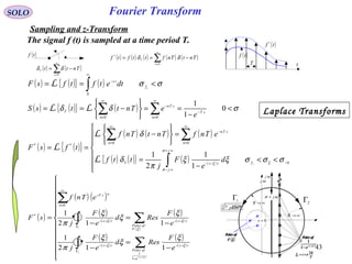
![55
Fourier TransformSOLO
The Discrete Time Fourier Transform (DTFT) (continue-2)
Normalization of the frequency
DTFT-1
DTFT
( ) ( )∑
+∞
−∞=
−
=
n
Tnfj
sDTFT
s
eTnsfS π2
: ( ) ( )
( )
( )
∫
+
−
=
s
s
s
T
T
nTfj
DTFTss dfefSTTns
2/1
2/1
2π
( ) ( )[ ]
[ ]2/1,2/1
2/1,2/1
:
*
*
+−∈
+−∈
=
f
TTf
Tff
ss
s
( ) ( )∑
+∞
−∞=
−
=
n
nfj
DTFT ensfS *2*
: π
DTFT-1
DTFT
( ) ( )∫
+
−
=
2/1
2/1
*2
** dfefSns nfj
DTFT
π
Example ( ) 1,,1,002
−== −
NneAns nfj
π
( ) ( )
( )
( )
( ) ( )
( ) ( )
( )
( )
( )[ ]
( )[ ]
( )( )1*
0
0
*
*
**
**
*2
*21
0
*2*
0
0
0
00
00
0
0
0
*sin
*sin
1
1
−−−
−−
−−
−−−
−−−
−−
−−−
=
−−
−
−
=
−
−
=
−
−
== ∑
Nffj
ffj
Nffj
ffjffj
NffjNffj
ffj
NffjN
n
nffj
DTFT
e
ff
Nff
A
e
e
ee
ee
A
e
e
AeAfS
π
π
π
ππ
ππ
π
π
π
π
π
|SDTFT(f*)|
Normalized Frequency](https://image.slidesharecdn.com/1-radarsignalprocessing-150117083950-conversion-gate01/85/1-radar-signal-processing-55-320.jpg)
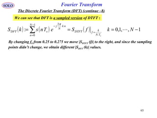
![57
Fourier Transform
( ) ( )∑
−
=
−
=
1
0
2
:
N
n
nk
N
j
sDFT eTnskS
π
SOLO
The Discrete Fourier Transform (DFT)
Assume a periodic sequence, sampled at a time period Ts, such that s (n Ts) = s [(n+kN) Ts]
The Discrete Fourier Transform (DFT) requires an input function that is discrete
and whose non-zero values have a limited (finite) duration.
Unlike the Discrete-time Fourier transform (DTFT), it only evaluates enough frequency
components to reconstruct the finite segment that was analyzed. Its inverse transform
cannot reproduce the entire time domain, unless the input happens to be periodic (forever).
Therefore it is often said that the DFT is a transform for Fourier analysis of finite-domain
discrete-time functions
For the sequence s (0), s (Ts),…,s [(N-1) Ts] we define the Discrete Fourier Transform:](https://image.slidesharecdn.com/1-radarsignalprocessing-150117083950-conversion-gate01/85/1-radar-signal-processing-57-320.jpg)
![58
Fourier Transform
( ) ( ) ( )∑∑
−
=
−
=
−
==
1
0
1
0
2
:
N
n
nk
s
N
n
nk
N
j
sDFT WTnseTnskS
π
SOLO
The Discrete Fourier Transform (DFT) (continue – 1)
For the sequence s (0), s (Ts),…,s [(N-1) Ts] we define the Discrete Fourier Transform:
where is a primitive N'th root of unity
and is periodic
N
j
eW
π2
:
−
=
n
Nm
N
j
n
N
j
Nmn
N
j
Nmn
WeeeW =
=
=
−−
+
−
+
1
222 πππ
( )
( )
( )
( )
( )
( ) ( ) ( ) ( ) ( )
( ) ( ) ( ) ( ) ( )
( ) ( ) ( ) ( ) ( )
( ) ( ) ( ) ( ) ( )
( ) ( ) ( ) ( ) ( )
[ ]
( )
( )
( )
( )[ ]
( )[ ]
N
N
N s
s
s
s
s
s
W
NNNNNNN
NNNNNNN
NN
NN
NN
S
DFT
DFT
DFT
DFT
DFT
TNs
TNs
Ts
Ts
Ts
WWWWW
WWWWW
WWWWW
WWWWW
WWWWW
NS
NS
S
S
S
⋅−
⋅−
⋅
⋅
⋅
=
−
−
−−−−−−−
−−−−−−−
−−
−−
−−
1
2
2
1
0
1
2
2
1
0
1121211101
1222221202
1222221202
1121211101
1020201000
[ ] NNN sWS = [ ]NW is a Vandermonde type of Matrix](https://image.slidesharecdn.com/1-radarsignalprocessing-150117083950-conversion-gate01/85/1-radar-signal-processing-58-320.jpg)
![59
Fourier TransformSOLO
The Discrete Fourier Transform (DFT) (continue – 2)
nNmn
WW =+
[ ] [ ] N
H
NN I
N
WW
1
=
N
j
eW
π2
−
= 1
2
* −
== WeW N
j
π
[ ]
( ) ( ) ( ) ( ) ( )
( ) ( ) ( ) ( ) ( )
( ) ( ) ( ) ( ) ( )
( ) ( ) ( ) ( ) ( )
( ) ( ) ( ) ( ) ( )
=
−−−−−−−
−−−−−−−
−−
−−
−−
1121211101
1222221202
1222221202
1121211101
1020201000
NNNNNNN
NNNNNNN
NN
NN
NN
N
WWWWW
WWWWW
WWWWW
WWWWW
WWWWW
W
[ ] [ ]
( ) ( ) ( ) ( ) ( )
( ) ( ) ( ) ( ) ( )
( ) ( ) ( ) ( ) ( )
( ) ( ) ( ) ( ) ( )
( ) ( ) ( ) ( ) ( )
==
−+−−+−−−−−−
−+−−+−−−−−−
+−+−−−
+−+−−−
+−+−−−
1112121110
2122222120
2122222120
1112121110
0102020100
*
NNNNNNN
NNNNNNN
NN
NN
NN
T
N
H
N
WWWWW
WWWWW
WWWWW
WWWWW
WWWWW
WW
Let multiply those two matrices
[ ] [ ]( )( ) ( ) ( ) ( ) ( ) ( ) ( ) ( ) ( )
( )
( )
( )
( )
( )
( )
=
≠=
−
−
=
−
−
==
+++++=
−
−
−
−−
=
−
+−−−−
∑
mkN
mk
W
W
W
W
W
WWWWWWWWWW
mk
mk
N
mk
NmkN
j
jmk
mNNkmjjkmkmk
mk
H
NN
0
1
1
1
1
1
1
0
111100
,
Where IN is the N x N identity matrix](https://image.slidesharecdn.com/1-radarsignalprocessing-150117083950-conversion-gate01/85/1-radar-signal-processing-59-320.jpg)
![60
Fourier Transform
( ) ( ) ( )∑∑
−
=
−
=
−
==
1
0
1
0
2
:
N
n
nk
s
N
n
nk
N
j
sDFT WTnseTnskS
π
SOLO
The Discrete Fourier Transform (DFT) (continue – 3)
For the sequence s (0), s (Ts),…,s [(N-1) Ts] we defined the Discrete Fourier Transform:
[ ] NNN sWS = [ ]NW is a Vandermonde type of Matrix
We found that
[ ] [ ] N
H
NN I
N
WW
1
= Where IN is the NxN identity matrix
Therefore the Inverse Discrete Fourier Transform (IDFT) is
[ ] N
H
NN SW
N
s
1
=
( ) ( ) ( )∑∑
−
=
−
=
−
==
1
0
21
0
11 N
n
nk
N
j
DFT
N
k
nk
DFTs ekS
N
WkS
N
Tns
π
D.F.T.
I.D.F.T.](https://image.slidesharecdn.com/1-radarsignalprocessing-150117083950-conversion-gate01/85/1-radar-signal-processing-60-320.jpg)
![61
Fourier TransformSOLO
The Discrete Fourier Transform (DFT) (continue – 4)
Second way to find the Inverse Discrete Fourier Transform (IDFT). Let compute:
( ) ( )
( )
( )
( )
∑ ∑∑∑∑
−
=
−
=
−−−
=
−
=
−−−
=
+
==
1
0
1
0
21
0
1
0
21
0
2 N
n
N
k
rnk
N
j
s
N
k
N
n
rnk
N
j
s
N
k
rk
N
j
DFT eTnseTnsekS
πππ
( )
( )
( )
( )
( )
( )[ ] ( )[ ]
( ) ( )
( )[ ]
( )
( )[ ] ( )[ ]
( ) ( )
( )[ ]
( )
( )
( )
( )[ ] ( )[ ]
( ) ( )
≠−
=−
=
−+
−
−+−
−
−
−
−
=
−+
−
−+−
−
−
=
−+
−−
−+−−
=
−
−
=
−
−
=
−−
−−
−−
−−
−
=
−−
∑
Nmrn
NmrnN
rn
N
jrn
N
rnjrn
rn
N
rn
N
rn
rn
N
rn
N
jrn
N
rnjrn
rn
N
rn
rn
N
jrn
N
rnjrn
e
e
e
e
e
rn
N
j
rnj
rn
N
j
N
rn
N
j
N
k
rnk
N
j
0
cossin
cossin
sin
sin
cossin
cossin
sin
sin
2
sin
2
cos1
2sin2cos1
1
1
1
1
2
2
2
2
1
0
2
ππ
ππ
π
π
π
π
ππ
ππ
π
π
ππ
ππ
π
π
π
π
π
( ) ( )[ ] ,2,1,0
1
0
2
±±=+=∑
−
=
+
mTmNrsNekS s
N
k
rk
N
j
DFT
π](https://image.slidesharecdn.com/1-radarsignalprocessing-150117083950-conversion-gate01/85/1-radar-signal-processing-61-320.jpg)
![62
Fourier Transform
( ) ( ) ( )∑∑
−
=
−
=
−
==
1
0
1
0
2
:
N
n
nk
s
N
n
nk
N
j
sDFT WTnseTnskS
π
SOLO
The Discrete Fourier Transform (DFT) (continue – 5)
For the sequence s (0), s (Ts),…,s [(N-1) Ts] we define the Discrete Fourier Transform:
where is a primitive N'th root of unity
and is periodic
N
j
eW
π2
:
−
=
n
Nm
N
j
n
N
j
Nmn
N
j
Nmn
WeeeW =
=
=
−−
+
−
+
1
222 πππ
( )
( )
( )
( )
( )
( )
( )
( )
( )[ ]
( )[ ]
⋅−
⋅−
⋅
⋅
⋅
=
−
−
−−
−−
−−
−−
s
s
s
s
s
NN
NN
NN
NN
DFT
DFT
DFT
DFT
DFT
TNs
TNs
Ts
Ts
Ts
WWWWW
WWWWW
WWWWW
WWWWW
WWWWW
NS
NS
S
S
S
1
2
2
1
0
1
2
2
1
0
12210
23320
23420
12210
00000
](https://image.slidesharecdn.com/1-radarsignalprocessing-150117083950-conversion-gate01/85/1-radar-signal-processing-62-320.jpg)
![63
Fourier TransformSOLO
The Discrete Fourier Transform (DFT) (continue – 6)
The DFT ant Inverse DFT (IDFT) are given by
( ) ( )∑
−
=
+
=
1
0
2
1 N
k
nk
N
j
DFTs ekS
N
Tns
π
( ) ( )∑
−
=
−
=
1
0
2
:
N
n
nk
N
j
sDFT eTnskS
π
IDFT
DFT
with the periodic properties
( )[ ] ( )
,2,1,0 ±±=
=+
m
TnsTmNns ss
( ) ( )
,2,1,0 ±±=
=+
m
kSNmkS DFTDFT
The sequence s (0), s (Ts),…,s [(N-1) Ts] can be interpreted to be a sequence of finite
length, given for r = 0, 1,…,N-1, and zero otherwise or a periodic sequence, defined
for all r.](https://image.slidesharecdn.com/1-radarsignalprocessing-150117083950-conversion-gate01/85/1-radar-signal-processing-63-320.jpg)
![64
Fourier Transform
( ) ( )∑
−
=
−
=
1
0
2
:
N
n
nk
N
j
sDFT eTnskS
π
SOLO
The Discrete Fourier Transform (DFT) (continue – 7)
The DFT ant Inverse DFT (IDFT) are given by
( ) ( )∑
−
=
+
=
1
0
2
1 N
k
nk
N
j
DFTs ekS
N
Tns
π
IDFT
DFT
( ) ( )∑
+∞
−∞=
−
=
n
nfj
DTFT ensfS *2*
: π
( ) ( )∫
+
−
=
2/1
2/1
*2
** dfefSns nfj
DTFT
π
IDTFT
DTFT
The DTFT ant Inverse DTFT (IDTFT) where given by
We can see that DFT is a sampled version of DTFT by tacking:
( ) ( )[ ]
[ ]2/1,2/1
2/1,2/1
1,,1,0
*
*
+−∈
+−∈
−==⇒==
f
TTf
Nk
TN
k
f
N
k
fTf
ss
s
s
( ) ( ) ( ) 1,,1,0:
1
0
2
−=== =
−
=
−
∑ NkfSeTnskS
sTN
k
fDTFT
N
n
nk
N
j
sDFT
π](https://image.slidesharecdn.com/1-radarsignalprocessing-150117083950-conversion-gate01/85/1-radar-signal-processing-64-320.jpg)
![72
SOLO
Properties of The Discrete Fourier Transform (DFT) (continue – 14)
( )mns − ( )
mk
N
j
DFT ekS
π2
−
Linearity1 ( ) ( )nsns 2211 αα +
Shift of a Sequence2
3
4
5
Periodic Convolution
6
7
Conjugate
8
9
IDFT
DFT ( ) ( )∑
−
=
−
=
1
0
2
:
N
n
nk
N
j
DFT enskS
π
( ) ( )∑
−
=
+
=
1
0
2
1 N
k
nk
N
j
DFT ekS
N
ns
π
( ) ( )kSkS DFTDFT 2211 αα +
( ) ( )nsns 21 , Periodic Sequence
(Period N)
( ) ( )kSkS DFTDFT 21 , DFT
(Period N)
( )
nl
N
j
ens
π2
−
( )lkSDFT −
( ) ( )∑
−
=
−⋅
1
0
21
N
m
mnsms
( ) ( )kSkS DFTDFT 21 ⋅
( ) ( )nsns 21 ⋅
( ) ( )∑
−
=
−⋅
1
0
21
1 N
l
DFTDFT lkSlS
N
( )ns∗
( )kSDFT −
∗
( )ns −∗
( )kSDFT
∗
Real & Imaginary ( )[ ]nsRe
( )[ ]nsImj
( ) ( ) ( )[ ] 2/kSkSkS DFTDFTeven −+=
∗
( ) ( ) ( )[ ] 2/kSkSkS DFTDFTodd −−=
∗](https://image.slidesharecdn.com/1-radarsignalprocessing-150117083950-conversion-gate01/85/1-radar-signal-processing-72-320.jpg)
![73
SOLO
Properties of The Discrete Fourier Transform (DFT) (continue – 15)
( ) ( ) ( )[ ] 2/: nsnsnseven −+= ∗
( )kSDFTReEven Part10
11
12 Symmetric Proprties
(only when s (n) is real)
IDFT
DFT ( ) ( )∑
−
=
−
=
1
0
2
:
N
n
nk
N
j
DFT enskS
π
( ) ( )∑
−
=
+
=
1
0
2
1 N
k
nk
N
j
DFT ekS
N
ns
π
( ) ( )nsns 21 , Periodic Sequence
(Period N)
( ) ( )kSkS DFTDFT 21 , DFT
(Period N)
( )lkSDFT −
( ) ( )
( )[ ] ( )[ ]
( )[ ] ( )[ ]
( ) ( )
( ) ( )
−−∠=∠
−=
−−=
−=
−=
∗
kSkS
kSkS
kSmkSm
kSkS
kSkS
DFTDFT
DFTDFT
DFTDFT
DFTDFT
DFTDFT
II
ReRe
Odd Part ( ) ( ) ( )[ ] 2/: nsnsnsodd −−= ∗
Return to Table of Content](https://image.slidesharecdn.com/1-radarsignalprocessing-150117083950-conversion-gate01/85/1-radar-signal-processing-73-320.jpg)
![75
Fourier TransformSOLO
Fast Fourier Transform (FFT)
The radix-2 DIT Algorithm
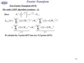
The radix-2 decimation-in-time (DIT) FFT is the simplest and most common form of the
Cooley-Tukey algorithm, although highly optimized Cooley-Tukey implementations
typically use other forms of the algorithm as described below. Radix-2 DIT divides a DFT
of size N into two interleaved DFTs (hence the name "radix-2") of size N/2 with each
recursive stage.
( ) ( ) ( )∑∑
−
=
−
=
−
==
1
0
1
0
2
:
N
n
nk
s
N
n
nk
N
j
sDFT WTnseTnskS
π
For the sequence s (0), s (Ts),…,s [(N-1) Ts] we define the Discrete Fourier Transform:
1,1, 22/1
2
*
2
+==−====→= −−−
−
ππ
ππ
jNj
evenN
NN
j
N
j
eWeWWeWeW
Suppose N is a power of 2; i.e. N=2L
(L is integer). Since N is a even integer, let compute
SDFT (k) by separate s (nTs) into two (N/2)-point sequences consisting of the even-numbered
points (n=2r) and odd numbered points (n=2r+1).
( ) ( )
( )
( ) ( )
( )
( ) ( )
( )
( ) ( )
( )
∑∑
∑∑
−
=
−
=
−
=
+
−
=
++=
++=
12/
0
2
12/
0
2
12/
0
12
12/
0
2
122
122
N
n
kr
N
k
N
N
n
kr
N
N
n
kr
N
N
n
kr
NDFT
WrsWWrs
WrsWrskS](https://image.slidesharecdn.com/1-radarsignalprocessing-150117083950-conversion-gate01/85/1-radar-signal-processing-75-320.jpg)
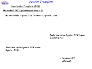
![79
Fourier TransformSOLO
Fast Fourier Transform (FFT)
The radix-2 DIT Algorithm (continue – 2)
( ) ( )kkj
kN
N
j
Nk
N eeW 1
2
2/
−==
= −
−
π
π
We divided the N-point DFT into two N/2-points DFTs.
( ) ( ) ( ) ( )
[ ]
( )
( ) ( )
( )
( )
∑∑
−
=
−
−
=
+
++=++=
12/
0
1
2/
12/
0
2/
2/2/
N
n
kn
N
Nk
N
N
n
Nnk
N
kn
NDFT WWNnsnsWNnsWnskS
k
Since N/2 is an even integer (N=2L
)
( ) ( ) ( )[ ]
( )
( )
( )
( )
( )
tgofFFTN
N
n
nl
N
WW
N
N
n
nl
N
ng
DFT WngWNnsnslkS
NN
L
2/
12/
0
2/
2
12/
0
2
2/
2
2/2 ∑∑
−
=
=
=
−
=
=++==
( ) ( ) ( )[ ]
( )
( )
( )
( )
( )
thofFFTN
N
n
nl
N
WW
N
N
n
nl
N
nh
n
NDFT WnhWWNnsnslkS
NN
L
2/
12/
0
2/
2
12/
0
2
2/
2
2/12 ∑∑
−
=
=
=
−
=
=+−=+=](https://image.slidesharecdn.com/1-radarsignalprocessing-150117083950-conversion-gate01/85/1-radar-signal-processing-79-320.jpg)
![83
Fourier TransformSOLO
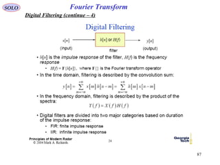
Digital Filtering
Digital Filters can be partitioned in two distinct classes:
• Finite Impulse Response (FIR) filters that have an impulse response
h (nT) of finite duration
( )
( )
≥<
−=
=
Nnn
Nnnh
Tnh
&,00
1,,1,0
• Infinite Impulse Response (IIR) filters that have an impulse response
h (nT) of infinite duration
If s (n) is an input signal to the digital filter, then the output of the digital filter
y (k) is related to the input by a relation of the type:
( ) ( ) ( )[ ] ( )[ ]
( )[ ] ( )[ ]TMkybTkyb
TNksaTksaTksaTky
M
N
−−−−−
−++−+=
1
1
1
10
If all the coefficients ai, bi are constants we can use the z transform to obtain:
( ) ( ) ( ) ( )zSzHzS
zbzb
zazaa
zY M
M
N
N
⋅=⋅
+++
+++
= −−
−−
1
1
1
10
1
For a causal filter N ≤ M.](https://image.slidesharecdn.com/1-radarsignalprocessing-150117083950-conversion-gate01/85/1-radar-signal-processing-83-320.jpg)
![92
Fourier TransformSOLO
Windowing
Rectangular [ ]
≤≤
=
otherwise
Mn
nw
,0
0,1
Bartlett
(triangular) [ ]
≤<−
≤≤
=
otherwise
MnMMn
MnMn
nw
,0
2/,/22
2/0,/2
Hanning
Hammming
[ ]
( )
≤≤−
=
otherwise
MnMn
nw
,0
0,/2cos5.05.0 π
[ ]
( )
≤≤−
=
otherwise
MnMn
nw
,0
0,/2cos46.054.0 π
Blackman [ ]
( ) ( )
≤≤+−
=
otherwise
MnMnMn
nw
,0
0,/4sin08.0/2cos5.042.0 ππ
Julius Ferdinand von Hann (1839 -1921)
Richard Wesley Hamming (1915 –1998)](https://image.slidesharecdn.com/1-radarsignalprocessing-150117083950-conversion-gate01/85/1-radar-signal-processing-92-320.jpg)
![93
Fourier TransformSOLO
Windowing (continue – 1)
cosine
[ ]
≤≤<
−
−
=
otherwise
Mn
M
Mn
nw
,0
0&5.0
2/
2/
2
1
exp
2
σ
σ
Lanczos
[ ]
≤≤
−
=
otherwise
Mn
M
n
nw
,0
0,1
2
sinc
Gauss
[ ]
≤≤
=
−
=
otherwise
Mn
M
n
M
n
nw
,0
0,sin
2
cos
πππ
[ ]
( )
≤≤
−−
=
otherwise
Mn
I
M
n
I
nw
,0
0,
1
2
1
0
2
0
α
α
Kaiser
α=2π
α=3π](https://image.slidesharecdn.com/1-radarsignalprocessing-150117083950-conversion-gate01/85/1-radar-signal-processing-93-320.jpg)
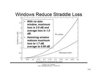
![95
Fourier TransformSOLO
Windowing (continue – 3)
Dolph-Chebyshev window
( ) ( )[ ]
( )
( )[ ]
( ) ( )4,3,2,10cosh
1
cosh
1,,2,1,0,
coshcosh
coscoscos
1
1
1
≈
=
−=
=
=
−
−
−
αβ
β
π
β
ω
ω
α
N
Nk
N
N
k
N
W
WIDFTnw
k
k
The α parameter controls the side-lobe level via the formula:
Side-Lobe Level in dB = - 20 α
The Dolph-Chebyshev Window (or Dolph window) minimizes the Chebyshev norm of
the side lobes for a given main lobe width 2 ωc:
( ) ( ){ }ωωω WWsidelobes cwwww >=∞= ∑
=
∑
maxmin:min 1,1,
The Chebyshev norm is also called the L - infinity norm, uniform norm, minimax
norm, or simply the maximum absolute value.](https://image.slidesharecdn.com/1-radarsignalprocessing-150117083950-conversion-gate01/85/1-radar-signal-processing-95-320.jpg)
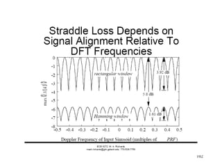
![109
SOLO Coherent Pulse Doppler Radar
An idealized target doppler response will
provide at IF Amplifier output the signal:
( ) ( )[ ] ( ) ( )
[ ]tjtj
dIFIF
dIFdIF
ee
A
tAts ωωωω
ωω +−+
+=+=
2
cos
that has the spectrum:
f
fIF+fd
-fIF-fd
-fIF fIF
A2
/4A2
/4 |s|2
0
Because we used N coherent pulses of
width τ and with Pulse Repetition Time T
the spectrum at the IF Amplifier output
f
-fd fd
A2
/4A2
/4
|s|2
0
After the mixer and base-band filter:
( ) ( ) [ ]tjtj
dd
dd
ee
A
tAts ωω
ω −
+==
2
cos
We can not distinguish between
positive to negative doppler!!!
and after the mixer :](https://image.slidesharecdn.com/1-radarsignalprocessing-150117083950-conversion-gate01/85/1-radar-signal-processing-109-320.jpg)
![110
SOLO Coherent Pulse Doppler Radar
We can not distinguish
between positive to negative
doppler!!!
Split IF Signal:
( ) ( )[ ] ( ) ( )
[ ]tjtj
dIFIF
dIFdIF
ee
A
tAts ωωωω
ωω +−+
+=+=
2
cos
( ) ( )[ ]
( ) ( )[ ]t
A
ts
t
A
ts
dIFQ
dIFI
ωω
ωω
+=
+=
sin
2
cos
2
Define a New Complex Signal:
( ) ( ) ( ) ( )[ ]tj
QI
dIF
e
A
tsjtstg ωω +
=+=
2
f
fIF+fd
fIF
A2
/2|g|2
0
f
fd
A2
/2
|s|2
0
Combining the signals after the mixers
( ) tj
d
d
e
A
tg ω
2
=
We now can distinguish
between positive to negative
doppler!!!](https://image.slidesharecdn.com/1-radarsignalprocessing-150117083950-conversion-gate01/85/1-radar-signal-processing-110-320.jpg)
![111
SOLO Coherent Pulse Doppler Radar
Split IF Signal:
( ) ( )[ ]
( ) ( )[ ]t
A
ts
t
A
ts
dIFQ
dIFI
ωω
ωω
+=
+=
sin
2
cos
2
Define a New Complex Signal:
( ) ( ) ( ) ( )[ ]tj
QI
dIF
e
A
tsjtstg ωω +
=+=
2
f
fd
A2
/2
|s|2
0
Combining the signals after the mixers
( ) tj
d
d
e
A
tg ω
2
=
We now can distinguish
between positive to negative
doppler!!!
From the Figure we can see that in this
case the doppler is unambiguous only if:
T
ff PRd
1
=<
Because we used N coherent pulses of
width τ and with Pulse Repetition Time T
the spectrum after the mixer output is
Return to Table of Content](https://image.slidesharecdn.com/1-radarsignalprocessing-150117083950-conversion-gate01/85/1-radar-signal-processing-111-320.jpg)
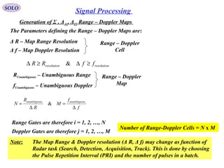
![119
SOLO Signal Processing
Generation of Σ , ΔAz, ΔEl Range – Doppler Maps (continue – 1)
The received signal from the scatter k is:
( ) ( )[ ] ( ) ( )ttTktttTkttfCts ddkdk
r
k
r
k ++≤≤++−= τθπ2cos
Ck
r
– amplitude of received signal
td (t) – round trip delay time given by ( )
2/c
tRR
tt kk
d
+
=
θk – relative phase
The received signal is down-converted to base-band in order to extract the quadrature
components. More precisely sk
r
(t) is mixed with: ( ) [ ] τθπ +≤≤+= TktTktfCty kkk 2cos
After Low-Pass filtering the quadrature components of Σk, ΔAz k or ΔEl k signals are:
( ) ( )
( ) ( )
=
=
tAtx
tAtx
kkQk
kkIk
ψ
ψ
sin
cos
( ) ( )
+−≅−=
c
tR
c
R
fttft kk
kdkk
22
22 ππψ
The quadrature samples are given by:
( ) ( )
+−≅=
c
tR
c
R
fjAjAtX kk
kkkkk
22
2expexp πψ
Ak - amplitude of Σk, ΔAz k or ΔEl k signals
ψk - phase of Σk, ΔAz k or ΔEl k signals
( )
+−
+≅+=
c
tR
c
R
fAj
c
tR
c
R
fAxjxtX kk
kk
kk
kkQkIkk
22
2sin
22
2cos ππ](https://image.slidesharecdn.com/1-radarsignalprocessing-150117083950-conversion-gate01/85/1-radar-signal-processing-119-320.jpg)
![130
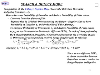
SOLO SEARCH & DETECT MODE
Computation of the Σ Range-Doppler Map, chooses the Detection Threshold
and policy (continue – 2).
DOPPLER
WINDOW
R W
A I
N N
G D
E O
W
R G
A A
N T
G E
E S
DOPPLER
FILTERS
S cells
CFAR
Window
R∆
f∆
Target
Uncertainty
Window
( ) ( ) ( )[ ]∑
∗
+ Σ⋅Σ=
n
j Window
CFARNoiseClutter jiji
n
iC ,,
1
Guard
(Gap)
Window
• Computation of Clutter + Noise Threshold
• Coherent Detection:
( ) ( )
( ) ( ) ClutterThjiNiCIf
ClutternoThjiNiCIf
NoiseClutter
NoiseClutter
⇒+>
⇒+≤
+
+
1,
1,
( ) NoiseThNjiS +≥
Window
yUncertaint
Target,
( ) ( ) ( )[ ]∑
∗
+ Σ⋅Σ=
n
j Window
CFARNoiseClutter jiji
n
iC ,,
1
1. If no Clutter declare a Detection in the (i,j) cell of the Target Window if
ThNoise is chosen to assure a predefined
Probability of Detection pd and of False Alarm pFA
( ) NoiseClutterNoiseClutter ThCjiS ++ +≥
Window
yUncertaint
Target,
2. If Clutter declare a Detection in the (i,j) cell of the Target Window if
ThNoise is chosen to assure a predefined
Probability of Detection pd and of False Alarm pFA](https://image.slidesharecdn.com/1-radarsignalprocessing-150117083950-conversion-gate01/85/1-radar-signal-processing-130-320.jpg)


The document covers radar signal processing concepts, including the generation and reception of radar signals, Fourier transforms, and Doppler effects. It discusses signal modulation, range estimation, and digital signal processing techniques used to detect targets. Various radar waveforms and types, as well as mathematical relationships in radar signal processing, are also explained.


![Polymer [ बहुलक ] Chemistry Notes PDF - Irfanullah Mehar - JJ Sir Chemistry.pdf](https://cdn.slidesharecdn.com/ss_thumbnails/polymerchemistrynotespdf-irfanullahmehar-jjsirchemistry-260210172118-3f9b37f7-thumbnail.jpg?width=640&height=640&fit=bounds)


