The document discusses performing a discrete wavelet transform (DWT) on a 1D signal using MATLAB. It loads a test signal, performs a 5-level DWT decomposition using the coif3 wavelet, then reconstructs the approximation and detail signals at each level. Plots of the original, approximation, and detail signals are generated.

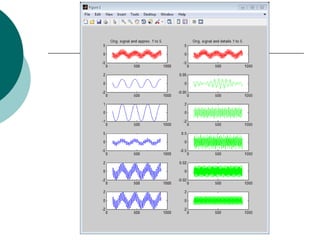
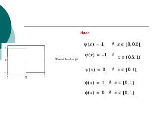
2. % Load original 1-D signal. 
load sumsin; s = sumsin; 

% Perform the decomposition of s at level 5, using coif3. 
w = 'coif3' 
[c,l] = wavedec(s,5,w); 

% Reconstruct the approximation signals and detail signals at 
% levels 1 to 5, using the wavelet decomposition structure [c,l]. 
for i = 1:5 
A(i,:) = wrcoef('a',c,l,w,i); 
D(i,:) = wrcoef('d',c,l,w,i); 
end 


% Plots. 
t = 100:900; 
subplot(6,2,1); plot(t,s(t),'r'); 
title('Orig. signal and approx. 1 to 5.'); 
subplot(6,2,2); plot(t,s(t),'r'); 
title('Orig. signal and details 1 to 5.'); 
for i = 1:5, 
subplot(6,2,2*i+1); plot(t,A(5-i+1,t),'b'); 
subplot(6,2,2*i+2); plot(t,D(5-i+1,t),'g'); 
end 

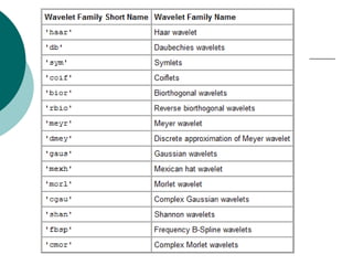
4. DWT Single-level discrete 1-D wavelet transform.
DWT performs a single-level 1-D wavelet decomposition
with respect to either a particular wavelet ('wname',
see WFILTERS for more information) or particular wavelet filters
(Lo_D and Hi_D) that you specify.
[CA,CD] = DWT(X,'wname') computes the approximation
coefficients vector CA and detail coefficients vector CD,
obtained by a wavelet decomposition of the vector X.
'wname' is a string containing the wavelet name.
[CA,CD] = DWT(X,Lo_D,Hi_D) computes the wavelet decomposition
as above given these filters as input:
Lo_D is the decomposition low-pass filter.
Hi_D is the decomposition high-pass filter.
Lo_D and Hi_D must be the same length.

5. Let LX = length(X) and LF = the length of filters; then
length(CA) = length(CD) = LA where LA = CEIL(LX/2),
if the DWT extension mode is set to periodization.
LA = FLOOR((LX+LF-1)/2) for the other extension modes.
For the different signal extension modes, see DWTMODE.
[CA,CD] = DWT(...,'mode',MODE) computes the wavelet
decomposition with the extension mode MODE you specify.
MODE is a string containing the extension mode.
Example:
x = 1:8;
[ca,cd] = dwt(x,'db1','mode','sym')

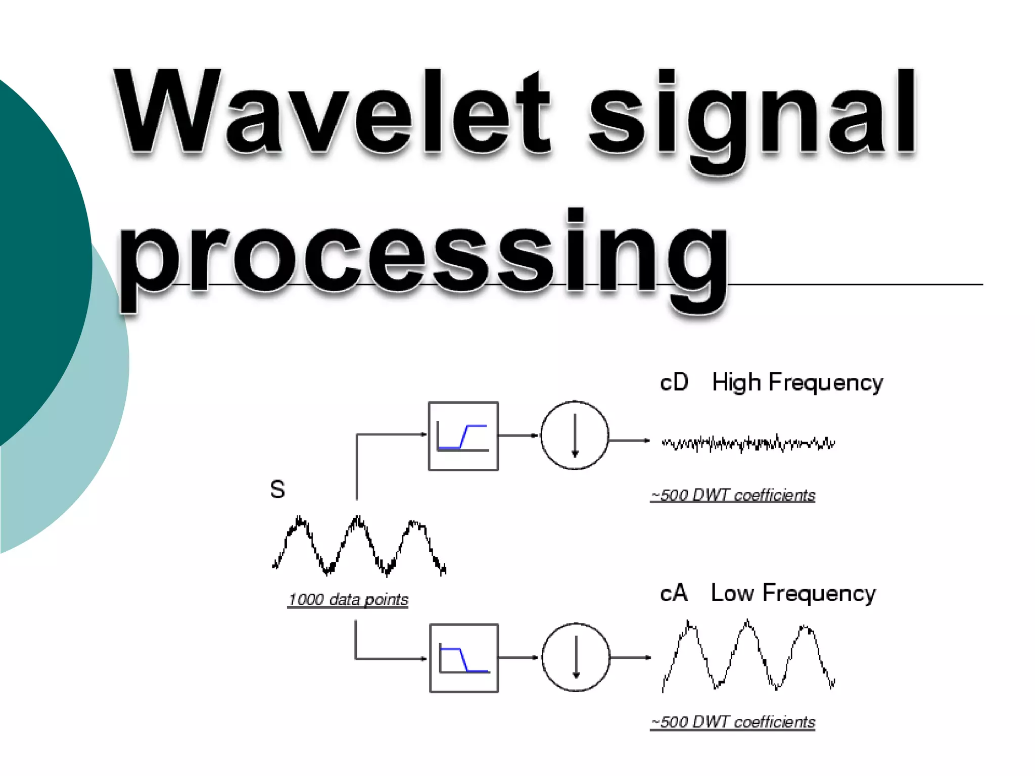
6. The MATLAB® code needed to generate s, cD, and cA is
s = sin(20.*linspace(0,pi,1000)) + 0.5.*rand(1,1000);
[cA,cD] = dwt(s,'db2');
where db2 is the name of the wavelet we want to use for the
analysis.
Notice that the detail coefficients cD are small and consist mainly of
a high-frequency noise, while the approximation coefficients cA
contain much less noise than does the original signal.
[length(cA) length(cD)] ans = 501 501

8. You may observe that the actual lengths of
the detail and approximation coefficient
vectors are slightly more than half the length
of the original signal. This has to do with the
filtering process, which is implemented by
convolving the signal with a filter. The
convolution "smears" the signal, introducing
several extra samples into the result.

9. Multistep Decomposition and
Reconstruction

10. This process involves two aspects: breaking up a signal to obtain 
the wavelet coefficients, and reassembling the signal from the
coefficients. 
We've already discussed decomposition and reconstruction at some
length. Of course, there is no point breaking up a signal merely to
have the satisfaction of immediately reconstructing it. We may
modify the wavelet coefficients before performing the reconstruction
step. We perform wavelet analysis because the coefficients thus
obtained have many known uses, de-noising and compression being
foremost among them.
But wavelet analysis is still a new and emerging field. No doubt, 
many uncharted uses of the wavelet coefficients lie in wait. The
toolbox can be a means of exploring possible uses and hitherto
unknown applications of wavelet analysis. Explore the toolbox
functions and see what you discover.

11. Wavelet Packet Analysis
The wavelet packet method is a generalization of 
wavelet decomposition that offers a richer range of
possibilities for signal analysis. 
In wavelet analysis, a signal is split into an
approximation and a detail. The approximation is then
itself split into a second-level approximation and detail,
and the process is repeated. For an n-level
decomposition, there are n+1 possible ways to
decompose or encode the signal.

13. In wavelet packet analysis, the details
as well as the approximations can be
split.

14. For instance, wavelet packet analysis allows the 
signal S to be represented as A1 + AAD3 + DAD3 +
DD2. This is an example of a representation that is
not possible with ordinary wavelet analysis.
Choosing one out of all these possible encodings
presents an interesting problem. In this toolbox, we
use an entropy-based criterion to select the most
suitable decomposition of a given signal. This means
we look at each node of the decomposition tree and
quantify the information to be gained by performing
each split.

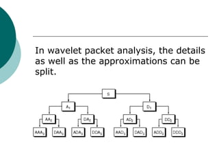
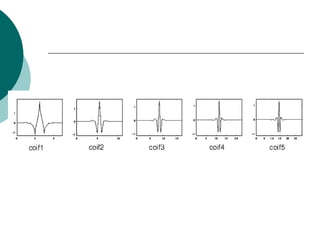
16. Simple and efficient algorithms exist for both wavelet
packet decomposition and optimal decomposition
selection. This toolbox uses an adaptive filtering
algorithm, based on work by Coifman and
Wickerhauser (see [CoiW92] in References), with direct
applications in optimal signal coding and data
compression.
Such algorithms allow the Wavelet Packet 1-D and
Wavelet Packet 2-D tools to include "Best Level" and
"Best Tree" features that optimize the decomposition
both globally and with respect to each node.

17. Introduction to the Wavelet
Families
Several families of wavelets that have
proven to be especially useful are
included in this toolbox. What follows
is an introduction to some wavelet
families.

18. Haar
Daubechies
Biorthogonal
Coiflets
Symlets
Morlet
Mexican Hat
Meyer
Other Real Wavelets
Complex Wavelets

19. Haar
Any discussion of wavelets begins
with Haar wavelet, the first and
simplest. Haar wavelet is
discontinuous, and resembles a step
function. It represents the same
wavelet as Daubechies db1. See Haar
for more detail.

22. >> mkdir C:worksl_hdlcoder_work
>> [cA1,cD1] = dwt(s,'db4');
>> [cA1,cD1] = dwt(s,'db12');
>> [cA2,cD2] = dwt(s,'haar');
>> plot(cA2)
>> plot(cD2)

23. cA2 plot

24. cD2 plot

25. Daubechies
Ingrid Daubechies, one of the brightest stars in the
world of wavelet research, invented what are called
compactly supported orthonormal wavelets -- thus
making discrete wavelet analysis practicable.
The names of the Daubechies family wavelets are
written dbN, where N is the order, and db the
"surname" of the wavelet. The db1 wavelet, as
mentioned above, is the same as Haar wavelet. Here
are the wavelet functions psi of the next nine members
of the family:

26. You can obtain a survey of the main properties of this family by typing
waveinfo('db') from the MATLAB command line. See Daubechies Wavelets: dbN for more detail.

27. dbN

28. waveinfo('db')
General characteristics: Compactly supported
wavelets with extremal phase and highest
number of vanishing moments for a given
support width. Associated scaling filters are
minimum-phase filters.
Family Daubechies
Short name db
Order N N strictly positive integer
Examples db1 or haar, db4, db15
Orthogonal yes
Biorthogonal yes
Compact support yes
DWT possible
CWT possible

29. Biorthogonal
This family of wavelets exhibits the
property of linear phase, which is
needed for signal and image
reconstruction. By using two
wavelets, one for decomposition (on
the left side) and the other for
reconstruction (on the right side)
instead of the same single one,
interesting properties are derived.

30. You can obtain a survey of the main properties of this family by typing
waveinfo('bior') from the MATLAB command line. See Biorthogonal Wavelet Pairs: biorNr.Nd for more detail.

31. Coiflets
Built by I. Daubechies at the request of R.
Coifman. The wavelet function has 2N
moments equal to 0 and the scaling function
has 2N-1 moments equal to 0. The two
functions have a support of length 6N-1. You
can obtain a survey of the main properties of
this family by typing waveinfo('coif') from the
MATLAB command line. See Coiflet Wavelets:
coifN for more detail.

33. Symlets
The symlets are nearly symmetrical
wavelets proposed by Daubechies as
modifications to the db family. The
properties of the two wavelet families
are similar. Here are the wavelet
functions psi.

34. You can obtain a survey of the main properties of this family by typing
waveinfo('sym') from the MATLAB command line. See Symlet Wavelets: symN for more detail.

35. Morlet
This wavelet has no scaling function,
but is explicit.

36. You can obtain a survey of the main
properties of this family by typing
waveinfo('morl') from the MATLAB
command line. See Morlet Wavelet:
morl for more detail.

37. Mexican Hat
This wavelet has no scaling function
and is derived from a function that is
proportional to the second derivative
function of the Gaussian probability
density function.

38. You can obtain a survey of the main properties of this family by typing
waveinfo('mexh') from the MATLAB command line. See Mexican Hat Wavelet: mexh for more information.

39. Meyer
The Meyer wavelet and scaling
function are defined in the frequency
domain.

40. You can obtain a survey of the main properties of this family by typing
waveinfo('meyer') from the MATLAB command line. See Meyer Wavelet: meyr for more detail.

41. Other Real Wavelets
Some other real wavelets are
available in the toolbox:
Reverse Biorthogonal
Gaussian derivatives family
FIR based approximation of the Meyer
wavelet
See Additional Real Wavelets for more
information.

42. Complex Wavelets
Some complex wavelet families are
available in the toolbox:
Gaussian derivatives
Morlet
Frequency B-Spline
Shannon
See Complex Wavelets for more
information.