- Daubechies wavelets are a family of orthogonal wavelets that provide the highest number of vanishing moments for a given width, defined through recursive equations. - They are approximately localized in both time and frequency domains. The wavelets and scaling functions are not defined by closed-form equations, but are instead generated numerically through an iterative process. - Properties include orthogonality, localization, and a maximal number of vanishing moments for a given support width, with more coefficients providing more moments. They are widely used for problems involving signal discontinuities or self-similarity.

2. Contents
• Definition.
• Daubechies wavelets.
• Coefficients for normalized Daub-4.
• Seeing the hidden - Plotting the Daubechies
wavelets.
• Steps for the construction.
• Properties of Daubechies Wavelets.
• Implementation.
• References.

3. Definition
• Sinusoidal functions are perfectly localized in the frequency
domain, but global in the spatial coordinate (position or time).
It is therefore difficult to represent a time or spatially limited
function in a Fourier basis.
• A wavelet basis however, is approximately localized in both
the frequency domain and the spatial domain. In addition to
this localization in both conjugate variables, we require that all
basis functions be mutually orthogonal and normalized.
• This places heavy restrictions on the allowable functions. In
the Daubechies formulation, these properties are achieved
through the process of recursion.
• The scaling functions and wavelets are defined recursively
through the use of dilation equations.

4. • The basic dilation equation is a two-scale or
dyadic difference equation:
• Φ(x) is known as the scaling function (or father
wavelet) and is the building block for the wavelet basis,
just as h _ 1(x) was in the Haar basis. The symbol N,
represents the order of the system and the Daubechies
basis of order N is denoted D N.
• Daubechies wavelets are localized in the temporal
domain, and approximately localized in the frequency
domain.

5. • Figure (1) shows the D4 scaling function and mother wavelet,
which coupled with the Fourier transform of the scaling
function.
• Equation (1) determines Φ(x) only up to a multiplicative
constant. The scaling function

6. • The wavelets Ψ( x) are defined in terms of the
scaling function, as in the Haar basis case. The
expression relating the mother wavelet to the
scaling function is
• Note that, where not explicitly indicated, the
integration limits are - ∞ to ∞.

7.  It is Daubechies, who gave solid foundation for
wavelet theory. She developed many wavelet system
with compact support (finite number of coefficients in
the refinement relation).
 In this section, we will explore one wavelet system
called Daub-4 type wavelet system. The peculiarity of
this wavelet system is that, there is no explicit function,
so we cannot draw it directly.
 What we are given is h(k)s, the coefficients in
refinement relation which connect Φ(t) and translates
of Φ(2t). These coefficients for normalized Daub-4 are
as follows:
DAUBECHIES WAVELETS

8. These coefficients for normalized
Daub-4 are as follows:

9. SEEING THE HIDDEN-PLOTTING THE
DAUBECHIES WAVELETS
• The problem here is that refinement relation tells us
how bigger scaling function can be expressed using
the smaller one. It does not tell us anyway how to
draw the bigger one or for that matter how to draw
the smaller one. Because of this, it has some parallel
with fractals.
• Many fractals have this nature. The whole is made up
of scaled and translated version of itself.
• For example, fern leaf as shown in Figure (a) This
fern leaf has no explicit equation to draw itself. Here
it is generated through an iterative scheme.

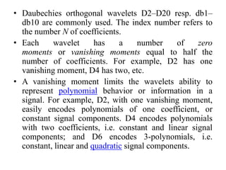
10. • To see Daubechies 4-tap wavelets, we will
initially use a brute force approach. Note that Φ(t)
of Daub-4 is defined in the range t = [O, 3]
because number of coefficients in the refinement
relation is 4. Φ(2t) lies in the range t = [O, 1.51.
Φ(2t - 1) lies in the range t = [0.5, 2].
• Similarly, Φ(2t - 2) in [ 1 , 2.5] and Φ(2t - 3) in
[1.5, 3]. Note again that four Φ(2t)s span the
range [O, 3].
• We now sample Φ(t ). Sample size must be
multiple of 2(N - I ) where N is the number of
coefficients.

11. • This is to place Φ(t)s properly in the given
range. Let us take sample size as 180, i.e., we
take 180 samples from Φ(t ).

12. Perform the following steps:
(i) Initialize arrays PHI20, PHI21,
PHI22, PHI23 of size 180 with
zeroes. Initialize array PHI of
size 180 with ones. Initialize
another array PHI2 of size 90
with zeroes.
(ii) Take alternate values from PHI array and fill
PHI2 array. (We are making Φ(2t) from Φ(t).)
(iii) Take PHI2 array. multiply with h(0) √2 and
store in PHI20 array from position 1 to 90.

13. iv) Take PHI2 array, multiply with h(1) ) √2 and store
in PHI21 array from position 31 to 120.
(v) Take PHI2 array, multiply with h(2)√2 and store in
PHI22 array from position 61 to 150.
(vi) Take PHI2 array, multiply with h(3) √2 and store
in PHI23 array from position 91 to 120.
(vii) Add PHI20, PHI21, PHI22, PHI23 array, point by
point, and store in PHI array.
(viii) Repeat steps from 2 to 7 several times (usually
within 10 iterations PHI array will
converge) and draw Φ(t). Figure (b) shows the
positioning of various array values.

15. (ix) Use converged Φ(t) values to draw Ψ( t ) using the
relation:
• Figure (c) shows the output of the above
procedure implemented in EXCEL
spreadsheet.
• The left figure is wavelet and the other is
scaling function.

17. Properties of Daubechies Wavelets
• The Daubechies wavelets, based on the work
of Ingrid Daubechies, are a family
of orthogonal wavelets defining a discrete
wavelet transform and characterized by a
maximal number of vanishing moments for
some given support. With each wavelet type of
this class, there is a scaling function (called
the father wavelet) which generates an
orthogonal multiresolution analysis.

18. • In general the Daubechies wavelets are chosen to have the
highest number A of vanishing moments, (this does not
imply the best smoothness) for given support width
2A − 1. There are two naming schemes in use, DN using
the length or number of taps, and dbA referring to the
number of vanishing moments. So D4 and db2 are the
same wavelet transform.
• Among the 2A−1 possible solutions of the algebraic
equations for the moment and orthogonality conditions,
the one is chosen whose scaling filter has extremal phase.
The wavelet transform is also easy to put into practice
using the fast wavelet transform. Daubechies wavelets are
widely used in solving a broad range of problems, e.g.
self-similarity properties of a signal or fractal problems,
signal discontinuities, etc.

19. • The Daubechies wavelets are not defined in terms
of the resulting scaling and wavelet functions; in
fact, they are not possible to write down in closed
form. The graphs below are generated using
the cascade algorithm, a numeric technique
consisting of simply inverse-transforming [1 0 0 0
0 ... ] an appropriate number of times.
• Note that the spectra shown here are not the
frequency response of the high and low pass
filters, but rather the amplitudes of the continuous
Fourier transforms of the scaling (blue) and
wavelet (red) functions.

21. • Daubechies orthogonal wavelets D2–D20 resp. db1–
db10 are commonly used. The index number refers to
the number N of coefficients.
• Each wavelet has a number of zero
moments or vanishing moments equal to half the
number of coefficients. For example, D2 has one
vanishing moment, D4 has two, etc.
• A vanishing moment limits the wavelets ability to
represent polynomial behavior or information in a
signal. For example, D2, with one vanishing moment,
easily encodes polynomials of one coefficient, or
constant signal components. D4 encodes polynomials
with two coefficients, i.e. constant and linear signal
components; and D6 encodes 3-polynomials, i.e.
constant, linear and quadratic signal components.

22. • This ability to encode signals is nonetheless
subject to the phenomenon of scale leakage, and
the lack of shift-invariance, which raise from the
discrete shifting operation (below) during
application of the transform. Sub-sequences
which represent linear, quadratic (for example)
signal components are treated differently by the
transform depending on whether the points align
with even- or odd-numbered locations in the
sequence.
• The lack of the important property of shift-
invariance, has led to the development of several
different versions of a shift-invariant (discrete)
wavelet transform.

23. Implementation
• While software such as Mathematica supports
Daubechies wavelets directly a basic implementation is
simple in MATLAB (in this case, Daubechies 4).
• This implementation uses periodization to handle the
problem of finite length signals. Other, more
sophisticated methods are available, but often it is not
necessary to use these as it only affects the very ends of
the transformed signal.
• The periodization is accomplished in the forward
transform directly in MATLAB vector notation, and the
inverse transform by using the circshift() function:

24. References
• Insight into wavelets from theory to practice by K.P.
Soman and K.I. Ramachandran.
• I. Daubechies, Ten Lectures on Wavelets, SIAM, 1992, p.
194.
• Daubechies Wavelet in Mathematica.
• Jensen; la Cour-Harbo (2001). Ripples in Mathematics.
Berlin: Springer. pp. 157–160. ISBN 3-540-41662-5.
• Jianhong (Jackie) Shen and Gilbert Strang, Applied and
Computational Harmonic Analysis, 5(3), Asymptotics of
Daubechies Filters, Scaling Functions, and Wavelets.

25. Thank U