This document discusses decision tree induction and attribute selection measures. It describes common measures like information gain, gain ratio, and Gini index that are used to select the best splitting attribute at each node in decision tree construction. It provides examples to illustrate information gain calculation for both discrete and continuous attributes. The document also discusses techniques for handling large datasets like SLIQ and SPRINT that build decision trees in a scalable manner by maintaining attribute value lists.

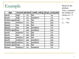
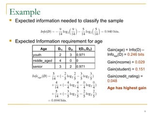
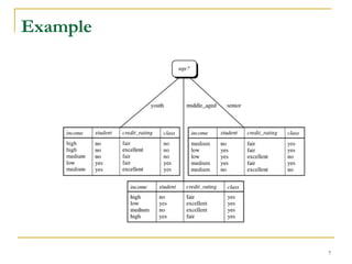
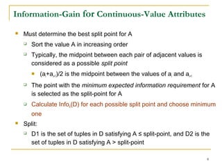
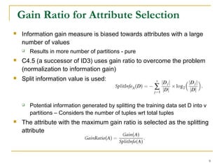
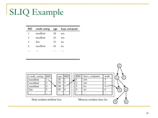
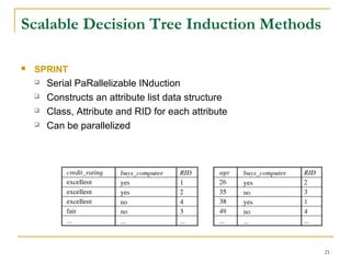
1. 1
Decision Tree Induction

2. 2
Attribute Selection Measures
 Heuristic for selecting splitting criterion
 Also termed as Splitting rules
 Ranks the attributes
 If selected attribute is continuous valued or discrete with binary split,
then split point or split subset must also be chosen
 Common measures – Information Gain, Gain ration, Gini Index
 Notations
 D – Data Partition
 Class label attribute has m distinct values – Ci 1=1..m
 Ci,D – Set of tuples of class i in D

3. 3
Attribute Selection Measure:
Information Gain
 Proposed by Claude Shannon
 Select the attribute with the highest information gain
 Minimizes the information needed to classify tuples in the resulting
partition
 Minimizes the expected number of tests needed to classify a tuple
 Expected information needed to classify a tuple in D
Info(D) = - ∑i=1
m
pi log2(pi)
where pi = |Ci,D|/|D| which is the probability that an arbitrary sample
belongs to class Ci
 Info(D) - Average information required to classify a tuple in D
 Info(D) is also known as entropy of D

4. 4
Information Gain
 Attribute A with v distinct values {a1, a2, …av}
 If A is discrete valued partition D into v subsets {D1,D2,…DV}
 Each partition is expected to be pure
 Additional information required to classify the samples is:
InfoA(D) = ∑j=1
v
|Dj| / |D| x Info(Dj)
 |Dj| / |D| - Weight of partition
 InfoA(D) – Expected information required to classify a tuple from D based
on partitioning by A
 Smaller the expected information greater the purity of partitions
 The Information Gain is given by:
Gain(A) = Info(D) – InfoA(D)
 Expected reduction in Information requirement by choosing A

5. 5
Example
Age income student credit_rating buys_computer
youth high no fair no
youth high no excellent no
middle-aged high no fair yes
senior medium no fair yes
senior low yes fair yes
senior low yes excellent no
middle-aged low yes excellent yes
youth medium no fair no
youth low yes fair yes
senior medium yes fair yes
youth medium yes excellent yes
middle-aged medium no excellent yes
middle-aged high yes fair yes
senior medium no excellent no
Based on the
attribute
‘buys_computer’
the number of
classes m = 2
C1 – ‘Yes’
C2 – ‘No’

6. 6
Example
 Expected information needed to classify the sample
 Expected Information requirement for age
Age D1i D2i I(D1i,D2i)
youth 2 3 0.971
middle_aged 4 0 0
senior 3 2 0.971
Gain(age) = Info(D) –
Infoage(D) = 0.246 bits
Gain(income) = 0.029
Gain(student) = 0.151
Gain(credit_rating) =
0.048
Age has highest gain

7. 7
Example

8. 8
Information-Gain for Continuous-Value Attributes
 Must determine the best split point for A
 Sort the value A in increasing order
 Typically, the midpoint between each pair of adjacent values is
considered as a possible split point
 (ai+ai+1)/2 is the midpoint between the values of ai and ai+1
 The point with the minimum expected information requirement for A
is selected as the split-point for A
 Calculate InfoA(D) for each possible split point and choose minimum
one
 Split:
 D1 is the set of tuples in D satisfying A ≤ split-point, and D2 is the
set of tuples in D satisfying A > split-point

9. 9
Gain Ratio for Attribute Selection
 Information gain measure is biased towards attributes with a large
number of values
 Results in more number of partitions - pure
 C4.5 (a successor of ID3) uses gain ratio to overcome the problem
(normalization to information gain)
 Split information value is used:
 Potential information generated by splitting the training data set D into v
partitions – Considers the number of tuples wrt total tuples
 The attribute with the maximum gain ratio is selected as the splitting
attribute

10. 10
Gain Ratio - Example
 Gain ratio for Income attribute
 Gain(Income) = 0.029
 GainRatio(Income) = 0.029/0.926 = 0.031

11. 11
Gini Index
 Measures the impurity of a data partition
 pj is probability of a tuple belonging to class Cj
 Considers a binary split for each value
 To determine best binary split on A, all possible subsets that can be
formed are considered
 2v
– 2 possible ways to form two partitions
 For binary splits
 Reduction in impurity
 Attribute that maximizes reduction in impurity or one with
minimum Gini index is chosen
∑
=
−=
n
j
p jDgini
1
21)(
)(
||
||
)(
||
||
)( 2
2
1
1
Dgini
D
D
Dgini
D
D
DginiA
+=
)()()( DginiDginiAgini A
−=∆

12. 12
Gini index
 Ex. D has 9 tuples in buys_computer = “yes” and 5 in “no”
 Suppose the attribute income partitions D into 10 in D1: {low,
medium} and 4 in D2
but gini{medium,high} is 0.30 and thus the best since it is the lowest
459.0
14
5
14
9
1)(
22
=





−





−=Dgini
)(
14
4
)(
14
10
)( 11},{ DGiniDGiniDgini mediumlowincome 





+





=∈

13. 13
Attribute Selection Measures
 The three measures, in general, return good results but
 Information gain:
 biased towards multivalued attributes
 Gain ratio:
 tends to prefer unbalanced splits in which one partition is much
smaller than the others
 Gini index:
 biased to multivalued attributes
 has difficulty when # of classes is large
 tends to favor tests that result in equal-sized partitions and
purity in both partitions

14. 14
Other Attribute Selection Measures
 CHAID: a popular decision tree algorithm, measure based on χ2
test
for independence
 C-SEP: performs better than info. gain and gini index in certain cases
 G-statistics: has a close approximation to χ2
distribution
 MDL (Minimal Description Length) principle (i.e., the simplest solution
is preferred):
 The best tree as the one that requires the fewest # of bits to both
(1) encode the tree, and (2) encode the exceptions to the tree
 Multivariate splits (partition based on multiple variable combinations)
 CART: finds multivariate splits based on a linear comb. of attrs.
 Best attribute selection measure
 Most give good results, none is significantly superior than others

15. 15
Overfitting and Tree Pruning
 Overfitting: An induced tree may overfit the training data
 Too many branches, some may reflect anomalies due to noise or outliers
 Poor accuracy for unseen samples
 Two approaches to avoid overfitting
 Prepruning: Halt tree construction early—do not split a node if this would
result in the goodness measure falling below a threshold
 Difficult to choose an appropriate threshold
 Postpruning: Remove branches from a “fully grown” tree—get a sequence
of progressively pruned trees
 Use a set of data different from the training data to decide which is the
“best pruned tree”

16. 16
Tree Pruning
 Cost Complexity pruning
 Post pruning approach used in CART
 Cost complexity – function of number of leaves and error rate of
the tree
 For each internal node cost complexity is calculated wrt original
and pruned versions
 If pruning results in a smaller cost complexity – subtree is pruned
 Uses a separate prune set
 Pessimistic Pruning
 Uses training set and adjusts error rates by adding a penalty
 Minimum Description Length (MDL) principle
 Issues: Repetition and Replication

17. 17
Enhancements to Basic Decision
Tree Induction
 Allow for continuous-valued attributes
 Dynamically define new discrete-valued attributes that partition the
continuous attribute value into a discrete set of intervals
 Handle missing attribute values
 Assign the most common value of the attribute
 Assign probability to each of the possible values
 Attribute construction
 Create new attributes based on existing ones that are sparsely
represented
 This reduces fragmentation, repetition, and replication

18. 18
Scalability and Decision Tree Induction
 Scalability: Classifying data sets with millions of examples and
hundreds of attributes with reasonable speed
 Large scale databases – do not fit into memory
 Repeated Swapping of data – Inefficient
 Scalable Variants
 SLIQ, SPRINT

19. 19
Scalable Decision Tree Induction
Methods
 SLIQ
 Supervised Learning in Quest
 Presort the data
 Builds an index for each attribute and only class list and the current
attribute list reside in memory
 Each attribute has an associated attribute list indexed by a Record
Identifier (RID) – linked to class list
 Class list points to node
 Limited by the size of the class list

20. 20
SLIQ Example

21. 21
Scalable Decision Tree Induction Methods
 SPRINT
 Serial PaRallelizable INduction
 Constructs an attribute list data structure
 Class, Attribute and RID for each attribute
 Can be parallelized

22. 22
Scalability Framework for RainForest
 Separates the scalability aspects from the criteria that determine
the quality of the tree
 Builds an AVC-list: AVC (Attribute, Value, Class_label)
 AVC-set (of an attribute X )
 Projection of training dataset onto the attribute X and class label
where counts of individual class label are aggregated

23. 23
Rainforest: Training Set and AVC Sets
student Buy_Computer
yes no
yes 6 1
no 3 4
Age Buy_Computer
yes no
<=30 3 2
31..40 4 0
>40 3 2
Credit
rating
Buy_Computer
yes no
fair 6 2
excellent 3 3
age income student
credit_
rating
buys_
comp
uter
<=30 high no fair no
<=30 high no excellent no
31…40 high no fair yes
>40 medium no fair yes
>40 low yes fair yes
>40 low yes excellent no
31…40 low yes excellent yes
<=30 medium no fair no
<=30 low yes fair yes
>40 medium yes fair yes
<=30 medium yes excellent yes
31…40 medium no excellent yes
31…40 high yes fair yes
>40 medium no excellent no
AVC-set on incomeAVC-set on Age
AVC-set on Student
Training Examples
income Buy_Computer
yes no
high 2 2
medium 4 2
low 3 1
AVC-set on
credit_rating

24. 24
BOAT (Bootstrapped Optimistic
Algorithm for Tree Construction)
 Use a statistical technique called bootstrapping to create several
smaller samples (subsets), each fits in memory
 Each subset is used to create a tree, resulting in several trees
 These trees are examined and used to construct a new tree T’
 It turns out that T’ is very close to the tree that would be generated
using the whole data set together
 Adv: requires only two scans of DB, an incremental algorithm
 Very much faster