Downloaded 124 times


![17
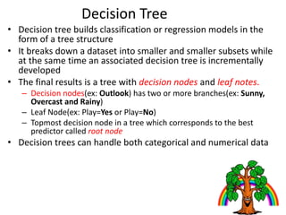
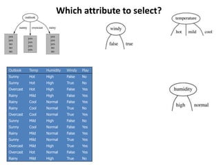
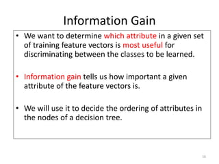
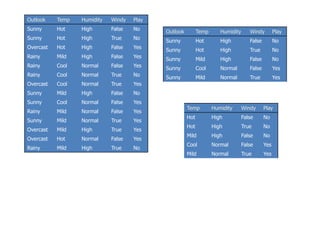
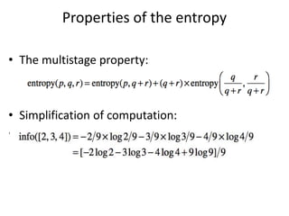
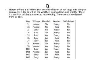
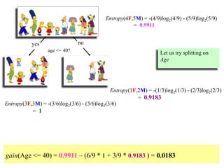
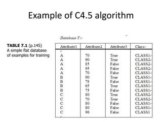
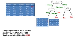
Calculating Information Gain
996.0
30
16
log
30
16
30
14
log
30
14
22
mpurity
787.0
17
4
log
17
4
17
13
log
17
13
22
impurity
Entire population (30 instances)
17 instances
13 instances
(Weighted) Average Entropy of Children = 615.0391.0
30
13
787.0
30
17
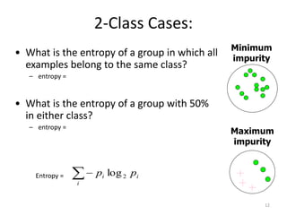
Information Gain= 0.996 - 0.615 = 0.38
391.0
13
12
log
13
12
13
1
log
13
1
22
impurity
Information Gain = entropy(parent) – [average entropy(children)]
gain(population)=info([14,16])-info([13,4],[1,12])
parent
entropy
child
entropy
child
entropy](https://image.slidesharecdn.com/decisiontree-160904075506/85/Decision-tree-17-320.jpg)
![18
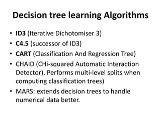
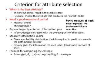
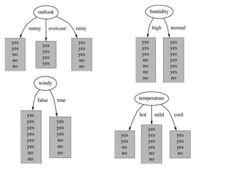
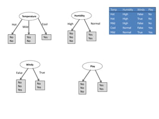
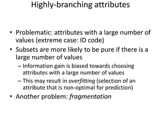
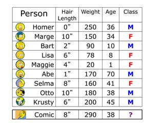
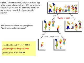
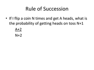
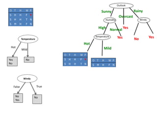
Calculating Information Gain
615.0391.0
30
13
787.0
30
17
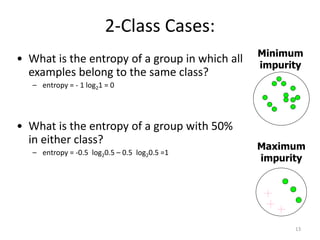
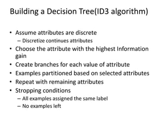
Information Gain= info([14,16])-info([13,4],[1,12])
= 0.996 - 0.615
= 0.38
391.0
13
12
log
13
12
13
1
log
13
1
22
impurity
Information Gain = entropy(parent) – [average entropy(children)]
gain(population)=info([14,16])-info([13,4],[1,12])
info[14/16]=entropy(14/30,16/30) =
info[13,4]=entropy(13/17,4/17) =
info[1.12]=entropy(1/13,12/13) =
996.0
30
16
log
30
16
30
14
log
30
14
22
impurity
787.0
17
4
log
17
4
17
13
log
17
13
22
impurity
info([13,4],[1,12]) =](https://image.slidesharecdn.com/decisiontree-160904075506/85/Decision-tree-18-320.jpg)

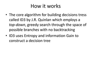
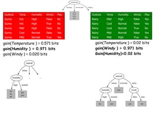
![Outlook = Sunny :
info[([2,3])=
Outlook = Overcast :
Info([4,0])=
Outlook = Rainy :
Info([2,3])=
i
ii pp 2log](https://image.slidesharecdn.com/decisiontree-160904075506/85/Decision-tree-21-320.jpg)
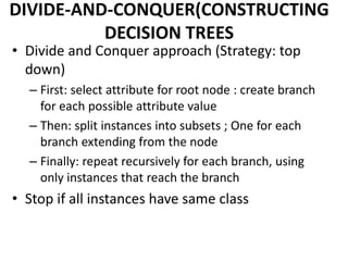
![Outlook = Sunny :
info[([2,3])=entropy(2/5,3/5)=
Outlook = Overcast :
Info([4,0])=entropy(1,0)=
Outlook = Rainy :
Info([2,3])=entropy(3/5,2/5)=
i
ii pp 2log](https://image.slidesharecdn.com/decisiontree-160904075506/85/Decision-tree-22-320.jpg)
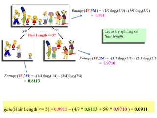
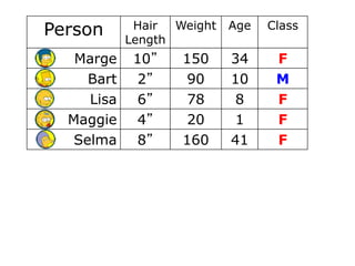
![Outlook = Sunny :
info[([2,3])=entropy(2/5,3/5)=−2/5log(2/5)−3/5log(3/5)=0.971bits
Outlook = Overcast :
Info([4,0])=entropy(1,0)=−1log(1)−0log(0)=0bits
Outlook = Rainy :
Info([2,3])=entropy(3/5,2/5)=−3/5log(3/5)−2/5log(2/5)=0.971bits
Expected information for attribute:
Info([3,2],[4,0],[3,2])=
Note: log(0) is normally
undefined but we
evaluate 0*log(0) as
zero
(Weighted) Average Entropy of Children =
i
ii pp 2log](https://image.slidesharecdn.com/decisiontree-160904075506/85/Decision-tree-23-320.jpg)
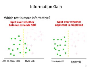
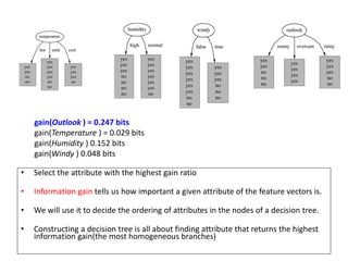
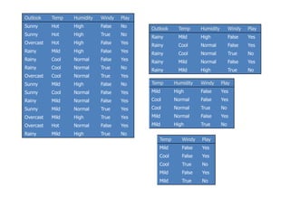
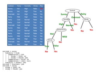
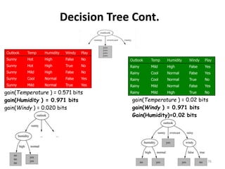
![Outlook = Sunny :
info[([2,3])=entropy(2/5,3/5)=−2/5log(2/5)−3/5log(3/5)=0.971bits
Outlook = Overcast :
Info([4,0])=entropy(1,0)=−1log(1)−0log(0)=0bits
Outlook = Rainy :
Info([2,3])=entropy(3/5,2/5)=−3/5log(3/5)−2/5log(2/5)=0.971bits
Expected information for attribute:
Info([3,2],[4,0],[3,2])=(5/14)×0.971+(4/14)×0+(5/14)×0.971=0.693bits
Information gain= information before splitting – information after splitting
gain(Outlook ) = info([9,5]) – info([2,3],[4,0],[3,2])
Note: log(0) is normally
undefined but we
evaluate 0*log(0) as
zero
i
ii pp 2log](https://image.slidesharecdn.com/decisiontree-160904075506/85/Decision-tree-24-320.jpg)
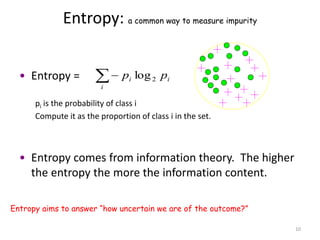
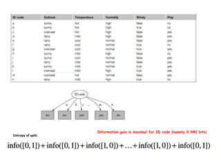
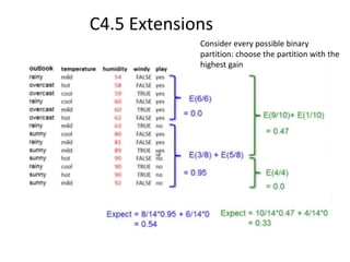
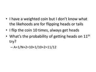
![Outlook = Sunny :
info[([2,3])=entropy(2/5,3/5)=−2/5log(2/5)−3/5log(3/5)=0.971bits
Outlook = Overcast :
Info([4,0])=entropy(1,0)=−1log(1)−0log(0)=0bits
Outlook = Rainy :
Info([2,3])=entropy(3/5,2/5)=−3/5log(3/5)−2/5log(2/5)=0.971bits
Expected information for attribute:
Info([3,2],[4,0],[3,2])=(5/14)×0.971+(4/14)×0+(5/14)×0.971=0.693bits
Information gain= information before splitting – information after splitting
gain(Outlook ) = info([9,5]) – info([2,3],[4,0],[3,2])
= 0.940 – 0.693
= 0.247 bits
Note: log(0) is normally
undefined but we
evaluate 0*log(0) as
zero](https://image.slidesharecdn.com/decisiontree-160904075506/85/Decision-tree-25-320.jpg)
![Humidity = high :
info[([3,4])=entropy(3/7,4/7)=−3/7log(3/7)−4/7log(4/7)=0.524+0.461=0.985 bits
Humidity = normal :
Info([6,1])=entropy(6/7,1/7)=−6/7log(6/7)−1/7log(1/7)=0.191+0.401=0.592 bits
Expected information for attribute:
Info([3,4],[6,1])=(7/14)×0.985+(7/14)×0.592=0.492+0.296= 0.788 bits
Information gain= information before splitting – information after splitting
gain(Humidity ) = info([9,5]) – info([3,4],[6,1])
= 0.940 – 0.788
= 0.152 bits](https://image.slidesharecdn.com/decisiontree-160904075506/85/Decision-tree-26-320.jpg)
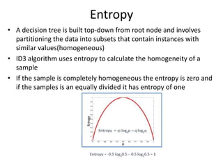
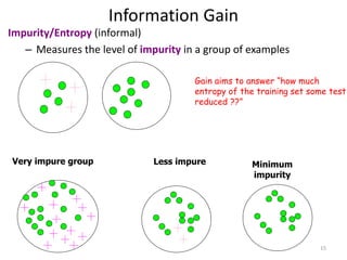
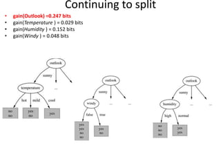
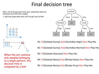
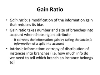
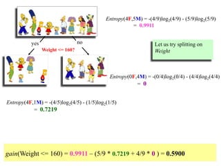
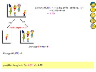
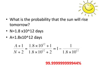
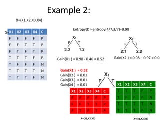
![gain(Outlook ) = 0.247 bits
gain(Temperature ) = 0.029 bits
gain(Humidity ) 0.152 bits
gain(Windy ) 0.048 bits
info(nodes)
=Info([2,3],[4,0],[3,2])
=0.693bits
gain= 0.940-0.693
= 0.247 bits
info(nodes)
=Info([6,2],[3,3])
=0.892 bits
gain=0.940-0.892
= 0.048 bits
info(nodes)
=Info([2,2],[4,2],[3,1])
=0.911 bits
gain=0.940-0.911
= 0.029 bits
info(nodes)
=Info([3,4],[6,1])
=0.788bits
gain= 0.940-0.788
=0.152 bits
Info(all features) =Info(9,5) =0.940 bits
This nodes is “pure” with only
“yes” pattern, therefore lower
entropy and higher gain](https://image.slidesharecdn.com/decisiontree-160904075506/85/Decision-tree-27-320.jpg)
![Temperature
No
No
Hot
Yes
No
Yes
Mild
Cool
Windy
No
No
Yes
False
No
Yes
True
Temperature = Hot :
info[([2,0])=entropy(1,0)=entropy(1,0)=−1log(1)−0log(0)=0 bits
Temperature = Mild :
Info([1,1])=entropy(1/2,1/2)=−1/2log(1/2)−1/2log(1/2)=0.5+0.5=1 bits
Temperature = Cool :
Info([1,0])=entropy(1,0)= 0 bits
Expected information for attribute:
Info([2,0],[1,1],[1,0])=(2/5)×0+(2/5)×1+(1/5)x0=0+0.4+0= 0.4 bits
gain(Temperature ) = info([3,2]) – info([2,0],[1,1],[1,0])
= 0.971-0.4= 0.571 bits
Play
No
No
No
Yes
Yes
Windy = False :
info[([2,1])=entropy(2/3,1/3)=−2/3log(2/3)−1/3log(1/3)=0.9179 bits
Windy = True :
Info([1,1])=entropy(1/2,1/2)=1 bits
Expected information for attribute:
Info([2,1],[1,1])=(3/5)×0.918+(2/5)×1=0.951bits
gain(Windy ) = info([3,2]) – info([2,1],[1,1])
= 0.971-0.951= 0.020 bits
Humidity
No
No
No
High
Yes
Yes
Normal
Humidity = High :
info[([3,0])=entropy(1,0)=0bits
Humidity = Normal :
Info([2,0])=entropy(1,0)=0 bits
Expected information for attribute:
Info([3,0],[2,0])=(3/5)×0+(2/5)×0=0 bits
gain(Humidity ) = info([3,2]) – Info([3,0],[2,0])
= 0.971-0= 0.971 bits
gain(Temperature ) = 0.571 bits
gain(Humidity ) = 0.971 bits
gain(Windy ) = 0.020 bits](https://image.slidesharecdn.com/decisiontree-160904075506/85/Decision-tree-32-320.jpg)
![Temp Windy Play
Mild False Yes
Cool False Yes
Cool True No
Mild False Yes
Mild True No
Temperature
---
Hot
Yes
Yes
No
Yes
No
Mild
Cool
Windy
Yes
Yes
Yes
False
No
No
True
Temperature = Mild :
Info([2,1])=entropy(1/2,1/2)=0.9179 bits
Temperature = Cool :
Info([1,1])=1 bits
Expected information for attribute:
Info([2,1],[1,1])=(3/5)×0.918+(2/5)×1=0.551+0.4= 0.951 bits
gain(Temperature ) = info([3,2]) – info([2,1],[1,1])
= 0.971-0.951= 0.02 bits
Play
Yes
Yes
Yes
No
No
Windy = False :
info[([3,0])=0 bits
Windy = True :
Info([2,0])=0 bits
Expected information for attribute:
Info([3,0],[2,0])= 0 bits
gain(Windy ) = info([3,2]) – info([3,0],[2,0])
= 0.971-0= 0.971 bits
gain(Temperature ) = 0.02 bits
gain(Windy ) = 0.971 bits](https://image.slidesharecdn.com/decisiontree-160904075506/85/Decision-tree-34-320.jpg)
![Wishlist for a purity measure
• Properties we require from a purity measure:
– When node is pure, measure should be zero
– When impurity is maximal (i.e. all classes equally likely),
measure should be maximal
– Measure should obey multistage property (i.e. decisions
can be made in several stages)
Measure ([ 2,3,4 ])=measure ([ 2,7 ]+(7 / 9)×measure
([ 3,4 ])
• Entropy is the only function that satisfies all three
properties!](https://image.slidesharecdn.com/decisiontree-160904075506/85/Decision-tree-36-320.jpg)
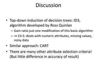
![Computing the gain ratio
• Example: intrinsic information for ID code
– Info([1,1,...,1])=14×(−1/14×log(1/14))=3.807bits
• Value of attribute decreases as intrinsic
information gets larger
• Definition of gain ratio:
gain_ratio(attribute)=gain(attribute)
intrinsic_info(attribute)
• Example:
gain_ratio(ID code)=0.940 bits =0.246
3.807 bits](https://image.slidesharecdn.com/decisiontree-160904075506/85/Decision-tree-41-320.jpg)
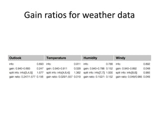

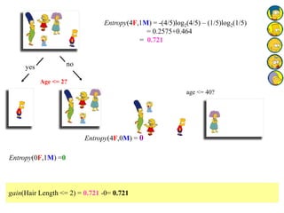
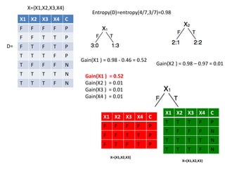


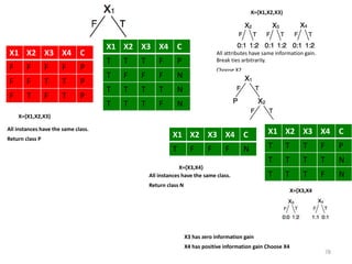
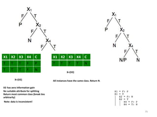
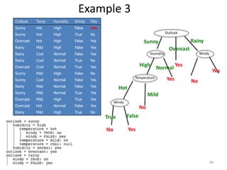


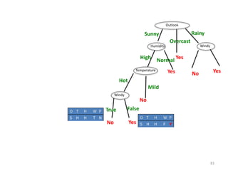
Decision trees are a machine learning technique that use a tree-like model to predict outcomes. They break down a dataset into smaller subsets based on attribute values. Decision trees evaluate attributes like outlook, temperature, humidity, and wind to determine the best predictor. The algorithm calculates information gain to determine which attribute best splits the data into the most homogeneous subsets. It selects the attribute with the highest information gain to place at the root node and then recursively builds the tree by splitting on subsequent attributes.