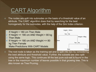
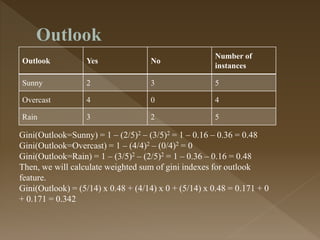
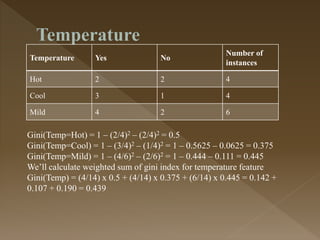
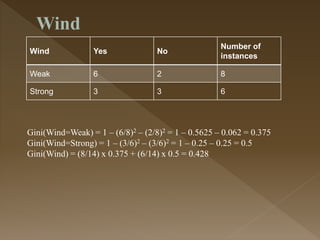
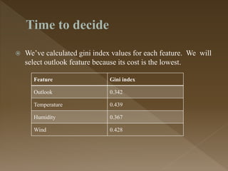
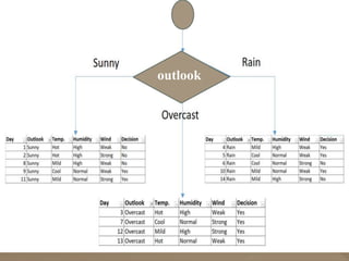
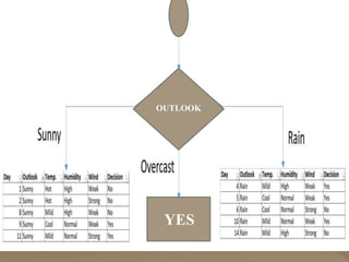
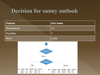
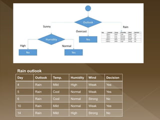
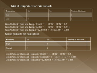
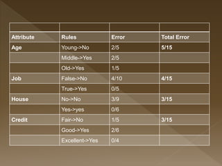
 Emaan Tahir-442
 Kaneez Amna-448
 Izza Shah-401
 Aiman Arshad-445
 Summaya Nazir-440
Presented To:
Ma’am Nazia
 1977: Breiman, Stone, Friedman, and Olshen invented the
first CART version. 1984: The official publication with a CART
decision tree software. It was a revolution in the world of
algorithms. Even today, CART is one of the most used
methods for decision tree data analytics.
 CART is an umbrella word that refers to the following types of
decision trees:
Classification Trees: When the target variable is continuous, the
tree is used to find the "class" into which the target variable is
most likely to fall.
Regression trees: These are used to forecast the value of a
continuous variable.
 The representation used for CART is a binary tree.
 Stopping criteria define how much tree learns and pruning can be
used to improve a learned tree.
 Predictions are made with CART by traversing the binary tree given
a new input record.
 The tree is learned using a greedy algorithm on the training data to
pick splits in the tree.
 The nodes are split into subnodes on the basis of a threshold value of an
attribute. The CART algorithm does that by searching for the best
homogeneity for the subnodes, with the help of the Gini Index criterion.
 The root node is taken as the training set and is split into two by considering
the best attribute and threshold value. Further, the subsets are also split
using the same logic. This continues till the last pure sub-set is found in the
tree or the maximum number of leaves possible in that growing tree. This is
also known as Tree Pruning.
1
2
3
4
If Height > 180 cm Then Male
If Height <= 180 cm AND Weight > 80 kg
Then Male
If Height <= 180 cm AND Weight <= 80
kg Then Female
Make Predictions With CART Models
Greedy Algorithm:
 The input variables and the split points are selected through a greedy
algorithm.
Stopping Criterion:
 The recursive binary splitting method described above must know
when to stop splitting. If the count is less than a certain threshold, the
split is rejected and the node is considered the last leaf node.
Tree pruning:
A decision tree's complexity is defined as the number of splits in the tree.
Only leaf nodes are eliminated if the total cost function for the complete
test set decreases.
EXAMPLE
Day Outlook Temp. Humidity Wind Decision
1 Sunny Hot High Weak No
2 Sunny Hot High Strong No
3 Overcast Hot High Weak Yes
4 Rain Mild High Weak Yes
5 Rain Cool Normal Weak Yes
6 Rain Cool Normal Strong No
7 Overcast Cool Normal Strong Yes
8 Sunny Mild High Weak No
9 Sunny Cool Normal Weak Yes
10 Rain Mild Normal Weak Yes
11 Sunny Mild Normal Strong Yes
12 Overcast Mild High Strong Yes
13 Overcast Hot Normal Weak Yes
14 Rain Mild High Strong No
Gini index is a metric for classification tasks in
CART. It stores sum of squared probabilities of
each class. We can formulate it as illustrated below.
Gini = 1 – Σ (Pi)2 for i=1 to number of classes
Outlook Yes No
Number of
instances
Sunny 2 3 5
Overcast 4 0 4
Rain 3 2 5
Gini(Outlook=Sunny) = 1 – (2/5)2 – (3/5)2 = 1 – 0.16 – 0.36 = 0.48
Gini(Outlook=Overcast) = 1 – (4/4)2 – (0/4)2 = 0
Gini(Outlook=Rain) = 1 – (3/5)2 – (2/5)2 = 1 – 0.36 – 0.16 = 0.48
Then, we will calculate weighted sum of gini indexes for outlook
feature.
Gini(Outlook) = (5/14) x 0.48 + (4/14) x 0 + (5/14) x 0.48 = 0.171 + 0
+ 0.171 = 0.342
Temperature Yes No
Number of
instances
Hot 2 2 4
Cool 3 1 4
Mild 4 2 6
Gini(Temp=Hot) = 1 – (2/4)2 – (2/4)2 = 0.5
Gini(Temp=Cool) = 1 – (3/4)2 – (1/4)2 = 1 – 0.5625 – 0.0625 = 0.375
Gini(Temp=Mild) = 1 – (4/6)2 – (2/6)2 = 1 – 0.444 – 0.111 = 0.445
We’ll calculate weighted sum of gini index for temperature feature
Gini(Temp) = (4/14) x 0.5 + (4/14) x 0.375 + (6/14) x 0.445 = 0.142 +
0.107 + 0.190 = 0.439
Humidity Yes No
Number of
instances
High 3 4 7
Normal 6 1 7
Gini(Humidity=High) = 1 – (3/7)2 – (4/7)2 = 1 – 0.183 – 0.326 =
0.489
Gini(Humidity=Normal) = 1 – (6/7)2 – (1/7)2 = 1 – 0.734 – 0.02 =
0.244
Weighted sum for humidity feature will be calculated next
Gini(Humidity) = (7/14) x 0.489 + (7/14) x 0.244 = 0.367
Wind Yes No
Number of
instances
Weak 6 2 8
Strong 3 3 6
Gini(Wind=Weak) = 1 – (6/8)2 – (2/8)2 = 1 – 0.5625 – 0.062 = 0.375
Gini(Wind=Strong) = 1 – (3/6)2 – (3/6)2 = 1 – 0.25 – 0.25 = 0.5
Gini(Wind) = (8/14) x 0.375 + (6/14) x 0.5 = 0.428
 We’ve calculated gini index values for each feature. We will
select outlook feature because its cost is the lowest.
Feature Gini index
Outlook 0.342
Temperature 0.439
Humidity 0.367
Wind 0.428
outlook
OUTLOOK
YES
Day Outlook Temp. Humidity Wind Decision
1 Sunny Hot High Weak No
2 Sunny Hot High Strong No
8 Sunny Mild High Weak No
9 Sunny Cool Normal Weak Yes
11 Sunny Mild Normal Strong Yes
Gini of temperature for sunny outlook
Temperature Yes No
Number of
instances
Hot 0 2 2
Cool 1 0 1
Mild 1 1 2
Gini(Outlook=Sunny and Temp.=Hot) = 1 – (0/2)2 – (2/2)2 = 0
Gini(Outlook=Sunny and Temp.=Cool) = 1 – (1/1)2 – (0/1)2 = 0
Gini(Outlook=Sunny and Temp.=Mild) = 1 – (1/2)2 – (1/2)2 = 1 – 0.25 – 0.25 = 0.5
Gini(Outlook=Sunny and Temp.) = (2/5)x0 + (1/5)x0 + (2/5)x0.5 = 0.2
Humidity Yes No Number of instances
High 0 3 3
Normal 2 0 2
Gini(Outlook=Sunny and Humidity=High) = 1 – (0/3)2 – (3/3)2 = 0
Gini(Outlook=Sunny and Humidity=Normal) = 1 – (2/2)2 – (0/2)2 = 0
Gini(Outlook=Sunny and Humidity) = (3/5)x0 + (2/5)x0 = 0
Gini of wind for sunny outlook
Wind Yes No
Number of
instances
Weak 1 2 3
Strong 1 1 2
Gini(Outlook=Sunny and Wind=Weak) = 1 – (1/3)2 – (2/3)2 = 0.266
Gini(Outlook=Sunny and Wind=Strong) = 1- (1/2)2 – (1/2)2 = 0.2
Gini(Outlook=Sunny and Wind) = (3/5)x0.266 + (2/5)x0.2 = 0.466
Feature Gini index
Temperature 0.2
Humidity 0
Wind 0.466
Rain outlook
Day Outlook Temp. Humidity Wind Decision
4 Rain Mild High Weak Yes
5 Rain Cool Normal Weak Yes
6 Rain Cool Normal Strong No
10 Rain Mild Normal Weak Yes
14 Rain Mild High Strong No
Temperature Yes No Number of instances
Cool 1 1 2
Mild 2 1 3
Gini(Outlook=Rain and Temp.=Cool) = 1 – (1/2)2 – (1/2)2 = 0.5
Gini(Outlook=Rain and Temp.=Mild) = 1 – (2/3)2 – (1/3)2 = 0.444
Gini(Outlook=Rain and Temp.) = (2/5)x0.5 + (3/5)x0.444 = 0.466
Gini of humidity for rain outlook
Humidity Yes No Number of instances
High 1 1 2
Normal 2 1 3
Gini(Outlook=Rain and Humidity=High) = 1 – (1/2)2 – (1/2)2 = 0.5
Gini(Outlook=Rain and Humidity=Normal) = 1 – (2/3)2 – (1/3)2 = 0.444
Gini(Outlook=Rain and Humidity) = (2/5)x0.5 + (3/5)x0.444 = 0.466
Wind Yes No Number of instances
Weak 3 0 3
Strong 0 2 2
Gini(Outlook=Rain and Wind=Weak) = 1 – (3/3)2 – (0/3)2 = 0
Gini(Outlook=Rain and Wind=Strong) = 1 – (0/2)2 – (2/2)2 = 0
Gini(Outlook=Rain and Wind) = (3/5)x0 + (2/5)x0 = 0
Decision for rain outlook
Feature Gini index
Temperature 0.466
Humidity 0.466
Wind 0
Example
Age Job House Credit Loan Approved
Young False No Fair No
Young False No Good No
Young True No Good Yes
Young True Yes Fair Yes
Young False No Fair No
Middle False No Fair No
Middle False No Good No
Middle True Yes Good Yes
Middle False Yes Excellent Yes
Old False Yes Excellent Yes
Old False Yes Good Yes
Old True No Good Yes
Old True No Excellent Yes
Young False No Good ?
Young 5 Yes 2
No 3
Middle 5 Yes 3
No 2
Old 5 Yes 4
No 1
individual error, and total for Age attribute
Attribute Rules Error Total Error
Age Young->No 2/5 5/15
Middle->Yes 2/5
Old->Yes 1/5
False 10 Yes 4
No 6
True 5 Yes 5
No 0
individual error, and total for Job attribute
Attribute Rules Error Total Error
Job False->No 4/10 4/15
True->Yes 0/5
No 9 Yes 3
No 6
Yes 6 Yes 6
No 0
individual error, and total for House attribute
Attribute Rules Error Total Error
House No->No 3/9 3/15
Yes->yes 0/6
Fair 5 Yes 1
No 4
Good 6 Yes 4
No 2
Excellent 4 Yes 4
No 0
individual error, and total for Credit attribute
Attribute Rules Error Total Error
Credit Fair->No 1/5 3/15
Good->Yes 2/6
Excellent->Yes 0/4
Attribute Rules Error Total Error
Age Young->No 2/5 5/15
Middle->Yes 2/5
Old->Yes 1/5
Job False->No 4/10 4/15
True->Yes 0/5
House No->No 3/9 3/15
Yes->yes 0/6
Credit Fair->No 1/5 3/15
Good->Yes 2/6
Excellent->Yes 0/4
House
YES
YES
NO
Age Job Credit LA
young False Fair No
Young False Good No
young True Good Yes
young False Fair No
Middle False Fair No
Middle False Good No
Old True Good Yes
Old True Excellent Yes
Old False Fair No
Attribute Rules Error Total Error
Age Young->No 1/4 2/9
Middle->No 0/2
Old->Yes 1/3
Job False->No 0/6 0/9
True->Yes 0/3
Credit Fair->No 0/4 2/9
Good->Yes/No 2/4
Excellent->Yes 0/1
House
YES
YES
YES
True
No
No
False
Job
Age Job House Credit
Loan
Approved
Young False No Good No
Advantages of CART Algorithm
 CART requires minimal supervision and produces easy-
to-understand models.
 It focuses on finding interactions and signal
discontinuity.
 It finds important variables automatically.
 It uses any combination of continuous/ discrete
variables.
Disadvantages of CART Algorithm
 This does not use combinations of variables.
 The tree structure may be unstable.
 It has a limited number of positions to accommodate
available predictors.
CART Algorithm.pptx
CART Algorithm.pptx

CART Algorithm.pptx

  • 2.
     Emaan Tahir-442 Kaneez Amna-448  Izza Shah-401  Aiman Arshad-445  Summaya Nazir-440 Presented To: Ma’am Nazia
  • 3.
     1977: Breiman,Stone, Friedman, and Olshen invented the first CART version. 1984: The official publication with a CART decision tree software. It was a revolution in the world of algorithms. Even today, CART is one of the most used methods for decision tree data analytics.  CART is an umbrella word that refers to the following types of decision trees: Classification Trees: When the target variable is continuous, the tree is used to find the "class" into which the target variable is most likely to fall. Regression trees: These are used to forecast the value of a continuous variable.
  • 4.
     The representationused for CART is a binary tree.  Stopping criteria define how much tree learns and pruning can be used to improve a learned tree.  Predictions are made with CART by traversing the binary tree given a new input record.  The tree is learned using a greedy algorithm on the training data to pick splits in the tree.
  • 5.
     The nodesare split into subnodes on the basis of a threshold value of an attribute. The CART algorithm does that by searching for the best homogeneity for the subnodes, with the help of the Gini Index criterion.  The root node is taken as the training set and is split into two by considering the best attribute and threshold value. Further, the subsets are also split using the same logic. This continues till the last pure sub-set is found in the tree or the maximum number of leaves possible in that growing tree. This is also known as Tree Pruning. 1 2 3 4 If Height > 180 cm Then Male If Height <= 180 cm AND Weight > 80 kg Then Male If Height <= 180 cm AND Weight <= 80 kg Then Female Make Predictions With CART Models
  • 6.
    Greedy Algorithm:  Theinput variables and the split points are selected through a greedy algorithm. Stopping Criterion:  The recursive binary splitting method described above must know when to stop splitting. If the count is less than a certain threshold, the split is rejected and the node is considered the last leaf node. Tree pruning: A decision tree's complexity is defined as the number of splits in the tree. Only leaf nodes are eliminated if the total cost function for the complete test set decreases.
  • 7.
  • 8.
    Day Outlook Temp.Humidity Wind Decision 1 Sunny Hot High Weak No 2 Sunny Hot High Strong No 3 Overcast Hot High Weak Yes 4 Rain Mild High Weak Yes 5 Rain Cool Normal Weak Yes 6 Rain Cool Normal Strong No 7 Overcast Cool Normal Strong Yes 8 Sunny Mild High Weak No 9 Sunny Cool Normal Weak Yes 10 Rain Mild Normal Weak Yes 11 Sunny Mild Normal Strong Yes 12 Overcast Mild High Strong Yes 13 Overcast Hot Normal Weak Yes 14 Rain Mild High Strong No
  • 9.
    Gini index isa metric for classification tasks in CART. It stores sum of squared probabilities of each class. We can formulate it as illustrated below. Gini = 1 – Σ (Pi)2 for i=1 to number of classes
  • 10.
    Outlook Yes No Numberof instances Sunny 2 3 5 Overcast 4 0 4 Rain 3 2 5 Gini(Outlook=Sunny) = 1 – (2/5)2 – (3/5)2 = 1 – 0.16 – 0.36 = 0.48 Gini(Outlook=Overcast) = 1 – (4/4)2 – (0/4)2 = 0 Gini(Outlook=Rain) = 1 – (3/5)2 – (2/5)2 = 1 – 0.36 – 0.16 = 0.48 Then, we will calculate weighted sum of gini indexes for outlook feature. Gini(Outlook) = (5/14) x 0.48 + (4/14) x 0 + (5/14) x 0.48 = 0.171 + 0 + 0.171 = 0.342
  • 11.
    Temperature Yes No Numberof instances Hot 2 2 4 Cool 3 1 4 Mild 4 2 6 Gini(Temp=Hot) = 1 – (2/4)2 – (2/4)2 = 0.5 Gini(Temp=Cool) = 1 – (3/4)2 – (1/4)2 = 1 – 0.5625 – 0.0625 = 0.375 Gini(Temp=Mild) = 1 – (4/6)2 – (2/6)2 = 1 – 0.444 – 0.111 = 0.445 We’ll calculate weighted sum of gini index for temperature feature Gini(Temp) = (4/14) x 0.5 + (4/14) x 0.375 + (6/14) x 0.445 = 0.142 + 0.107 + 0.190 = 0.439
  • 12.
    Humidity Yes No Numberof instances High 3 4 7 Normal 6 1 7 Gini(Humidity=High) = 1 – (3/7)2 – (4/7)2 = 1 – 0.183 – 0.326 = 0.489 Gini(Humidity=Normal) = 1 – (6/7)2 – (1/7)2 = 1 – 0.734 – 0.02 = 0.244 Weighted sum for humidity feature will be calculated next Gini(Humidity) = (7/14) x 0.489 + (7/14) x 0.244 = 0.367
  • 13.
    Wind Yes No Numberof instances Weak 6 2 8 Strong 3 3 6 Gini(Wind=Weak) = 1 – (6/8)2 – (2/8)2 = 1 – 0.5625 – 0.062 = 0.375 Gini(Wind=Strong) = 1 – (3/6)2 – (3/6)2 = 1 – 0.25 – 0.25 = 0.5 Gini(Wind) = (8/14) x 0.375 + (6/14) x 0.5 = 0.428
  • 14.
     We’ve calculatedgini index values for each feature. We will select outlook feature because its cost is the lowest. Feature Gini index Outlook 0.342 Temperature 0.439 Humidity 0.367 Wind 0.428
  • 15.
  • 16.
  • 17.
    Day Outlook Temp.Humidity Wind Decision 1 Sunny Hot High Weak No 2 Sunny Hot High Strong No 8 Sunny Mild High Weak No 9 Sunny Cool Normal Weak Yes 11 Sunny Mild Normal Strong Yes Gini of temperature for sunny outlook Temperature Yes No Number of instances Hot 0 2 2 Cool 1 0 1 Mild 1 1 2 Gini(Outlook=Sunny and Temp.=Hot) = 1 – (0/2)2 – (2/2)2 = 0 Gini(Outlook=Sunny and Temp.=Cool) = 1 – (1/1)2 – (0/1)2 = 0 Gini(Outlook=Sunny and Temp.=Mild) = 1 – (1/2)2 – (1/2)2 = 1 – 0.25 – 0.25 = 0.5 Gini(Outlook=Sunny and Temp.) = (2/5)x0 + (1/5)x0 + (2/5)x0.5 = 0.2
  • 18.
    Humidity Yes NoNumber of instances High 0 3 3 Normal 2 0 2 Gini(Outlook=Sunny and Humidity=High) = 1 – (0/3)2 – (3/3)2 = 0 Gini(Outlook=Sunny and Humidity=Normal) = 1 – (2/2)2 – (0/2)2 = 0 Gini(Outlook=Sunny and Humidity) = (3/5)x0 + (2/5)x0 = 0 Gini of wind for sunny outlook Wind Yes No Number of instances Weak 1 2 3 Strong 1 1 2 Gini(Outlook=Sunny and Wind=Weak) = 1 – (1/3)2 – (2/3)2 = 0.266 Gini(Outlook=Sunny and Wind=Strong) = 1- (1/2)2 – (1/2)2 = 0.2 Gini(Outlook=Sunny and Wind) = (3/5)x0.266 + (2/5)x0.2 = 0.466
  • 19.
    Feature Gini index Temperature0.2 Humidity 0 Wind 0.466
  • 20.
    Rain outlook Day OutlookTemp. Humidity Wind Decision 4 Rain Mild High Weak Yes 5 Rain Cool Normal Weak Yes 6 Rain Cool Normal Strong No 10 Rain Mild Normal Weak Yes 14 Rain Mild High Strong No
  • 21.
    Temperature Yes NoNumber of instances Cool 1 1 2 Mild 2 1 3 Gini(Outlook=Rain and Temp.=Cool) = 1 – (1/2)2 – (1/2)2 = 0.5 Gini(Outlook=Rain and Temp.=Mild) = 1 – (2/3)2 – (1/3)2 = 0.444 Gini(Outlook=Rain and Temp.) = (2/5)x0.5 + (3/5)x0.444 = 0.466 Gini of humidity for rain outlook Humidity Yes No Number of instances High 1 1 2 Normal 2 1 3 Gini(Outlook=Rain and Humidity=High) = 1 – (1/2)2 – (1/2)2 = 0.5 Gini(Outlook=Rain and Humidity=Normal) = 1 – (2/3)2 – (1/3)2 = 0.444 Gini(Outlook=Rain and Humidity) = (2/5)x0.5 + (3/5)x0.444 = 0.466
  • 22.
    Wind Yes NoNumber of instances Weak 3 0 3 Strong 0 2 2 Gini(Outlook=Rain and Wind=Weak) = 1 – (3/3)2 – (0/3)2 = 0 Gini(Outlook=Rain and Wind=Strong) = 1 – (0/2)2 – (2/2)2 = 0 Gini(Outlook=Rain and Wind) = (3/5)x0 + (2/5)x0 = 0 Decision for rain outlook Feature Gini index Temperature 0.466 Humidity 0.466 Wind 0
  • 24.
  • 25.
    Age Job HouseCredit Loan Approved Young False No Fair No Young False No Good No Young True No Good Yes Young True Yes Fair Yes Young False No Fair No Middle False No Fair No Middle False No Good No Middle True Yes Good Yes Middle False Yes Excellent Yes Middle False Yes Excellent Yes Old False Yes Excellent Yes Old False Yes Good Yes Old True No Good Yes Old True No Excellent Yes Young False No Good ?
  • 26.
    Young 5 Yes2 No 3 Middle 5 Yes 3 No 2 Old 5 Yes 4 No 1 individual error, and total for Age attribute Attribute Rules Error Total Error Age Young->No 2/5 5/15 Middle->Yes 2/5 Old->Yes 1/5
  • 27.
    False 10 Yes4 No 6 True 5 Yes 5 No 0 individual error, and total for Job attribute Attribute Rules Error Total Error Job False->No 4/10 4/15 True->Yes 0/5
  • 28.
    No 9 Yes3 No 6 Yes 6 Yes 6 No 0 individual error, and total for House attribute Attribute Rules Error Total Error House No->No 3/9 3/15 Yes->yes 0/6
  • 29.
    Fair 5 Yes1 No 4 Good 6 Yes 4 No 2 Excellent 4 Yes 4 No 0 individual error, and total for Credit attribute Attribute Rules Error Total Error Credit Fair->No 1/5 3/15 Good->Yes 2/6 Excellent->Yes 0/4
  • 30.
    Attribute Rules ErrorTotal Error Age Young->No 2/5 5/15 Middle->Yes 2/5 Old->Yes 1/5 Job False->No 4/10 4/15 True->Yes 0/5 House No->No 3/9 3/15 Yes->yes 0/6 Credit Fair->No 1/5 3/15 Good->Yes 2/6 Excellent->Yes 0/4
  • 31.
    House YES YES NO Age Job CreditLA young False Fair No Young False Good No young True Good Yes young False Fair No Middle False Fair No Middle False Good No Old True Good Yes Old True Excellent Yes Old False Fair No
  • 32.
    Attribute Rules ErrorTotal Error Age Young->No 1/4 2/9 Middle->No 0/2 Old->Yes 1/3 Job False->No 0/6 0/9 True->Yes 0/3 Credit Fair->No 0/4 2/9 Good->Yes/No 2/4 Excellent->Yes 0/1
  • 33.
    House YES YES YES True No No False Job Age Job HouseCredit Loan Approved Young False No Good No
  • 36.
    Advantages of CARTAlgorithm  CART requires minimal supervision and produces easy- to-understand models.  It focuses on finding interactions and signal discontinuity.  It finds important variables automatically.  It uses any combination of continuous/ discrete variables. Disadvantages of CART Algorithm  This does not use combinations of variables.  The tree structure may be unstable.  It has a limited number of positions to accommodate available predictors.