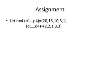
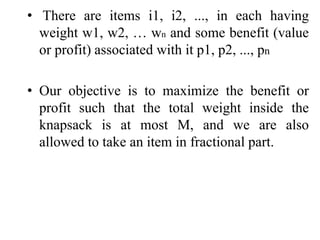
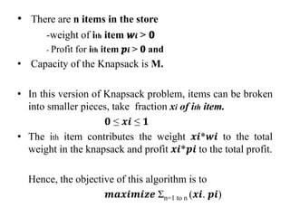
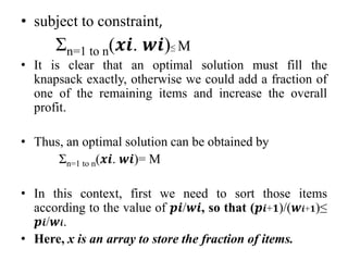
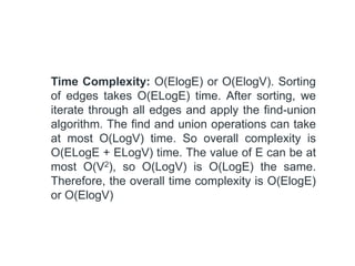
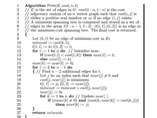
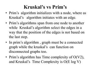
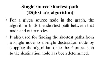
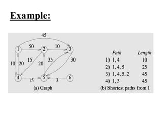
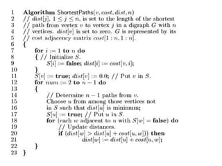
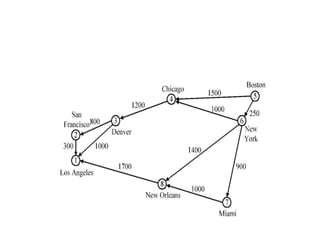
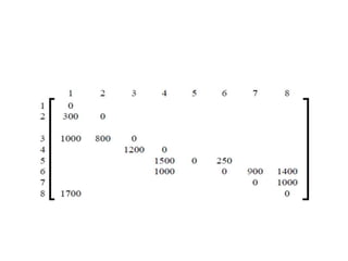
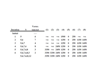
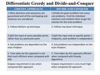
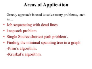
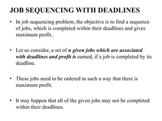
The document discusses the greedy method algorithmic approach. It provides an overview of greedy algorithms including that they make locally optimal choices at each step to find a global optimal solution. The document also provides examples of problems that can be solved using greedy methods like job sequencing, the knapsack problem, finding minimum spanning trees, and single source shortest paths. It summarizes control flow and applications of greedy algorithms.

1. UNIT - 3
Greedy Method

2. • Among all the algorithmic approaches, the simplest and
straightforward approach is the Greedy method.
• In this approach, the decision is taken on the basis of
current available information without worrying about the
effect of the current decision in future.
• Greedy algorithms build a solution part by part, choosing
the next part in such a way, that it gives an immediate
benefit.
• This approach never reconsiders the choices taken
previously

3. • This approach is mainly used to solve optimization
problems.
• Greedy method is easy to implement and quite efficient
in most of the cases.
• Greedy algorithm is an algorithmic paradigm based on
heuristic that follows local optimal choice at each step
with the hope of finding global optimal solution.
• In many problems, it does not produce an optimal
solution though it gives an approximate (near optimal)
solution in a reasonable time.

4. Control abstraction for Greedy Method
Algorithm GreedyMethod (a, n)
{
// a is an array of n inputs
Solution: =Ø;
for i: =0 to n do
{
s: = select (a);
if (feasible (Solution, s)) then
{
Solution: = union (Solution, s);
}
else reject (); // if solution is not feasible reject it.
}
return solution;
}

5. Three important activities
1. A selection of solution from the given input domain
is performed, i.e. s:= select(a).
2. The feasibility of the solution is performed, by using
feasible ‘(solution, s)’ and then all feasible solutions
are obtained.
3. From the set of feasible solutions, the particular
solution that minimizes or maximizes the given
objection function is obtained. Such a solution is
called optimal solution.

6. Differentiate Greedy and Divide-and-Conquer
GREEDY APPROACH DIVIDE AND CONQUER
1.Many decisions and sequences are
guaranteed and all the overlapping sub-
instances are considered.
1.Divide the given problem into many
sub problems. Find the individual
solutions and combine them to get the
solution for the main problem
2. Follows Bottom-up technique 2. Follows top down technique
3.Split the input at every possible points
rather than at a particular point
3.Split the input only at specific points (
midpoint), each problem is independent.
4. Sub problems are dependent on the
main Problem
4. Sub problems are independent on the
main Problem
5. Time taken by this approach is not
that much efficient when compared with
DAC
5. Time taken by this approach efficient
when compared with Greedy
Algorithms.
6.Space requirement is less when
compared DAC approach.
6.Space requirement is very much high
when compared GA approach.

7. Areas of Application
Greedy approach is used to solve many problems, such
as…
• Job sequencing with dead lines
• knapsack problem
• Single Source shortest path problem .
• Finding the minimal spanning tree in a graph
-Prim’s algorithm,
-Kruskal’s algorithm.

8. JOB SEQUENCING WITH DEADLINES
• In job sequencing problem, the objective is to find a sequence
of jobs, which is completed within their deadlines and gives
maximum profit..
• Let us consider, a set of n given jobs which are associated
with deadlines and profit is earned, if a job is completed by its
deadline.
• These jobs need to be ordered in such a way that there is
maximum profit.
• It may happen that all of the given jobs may not be completed
within their deadlines.

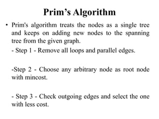
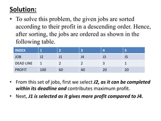
9. • Assume, deadline of ith job Ji is di and the profit
received from this job is pi. Hence, the optimal
solution of this algorithm is a feasible solution
with maximum profit.
• Thus, 𝑫(𝒊) > 𝟎 for 𝟏 ≤ 𝒊 ≤ 𝒏.
• Initially, these jobs are ordered according to profit,
i.e. 𝒑𝟏 ≥ 𝒑𝟐 ≥ 𝒑𝟑 ≥ … ≥ 𝒑𝒏.
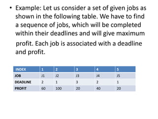
Ex: J=[j1,j2,j3,j4] P=[100,27,15,10], D= [2,1,2,1]
J=[j1,j2,j3,j4,j5] P=[20,15,10,5,1], D= [2,2,1,3,3]

10. • Example: Let us consider a set of given jobs as
shown in the following table. We have to find
a sequence of jobs, which will be completed
within their deadlines and will give maximum
profit. Each job is associated with a deadline
and profit.
INDEX 1 2 3 4 5
JOB J1 J2 J3 J4 J5
DEADLINE 2 1 3 2 1
PROFIT 60 100 20 40 20

11. Solution:
• To solve this problem, the given jobs are sorted
according to their profit in a descending order. Hence,
after sorting, the jobs are ordered as shown in the
following table.
• From this set of jobs, first we select J2, as it can be completed
within its deadline and contributes maximum profit.
• Next, J1 is selected as it gives more profit compared to J4.
INDEX 1 2 3 4 5
JOB J2 J1 J4 J3 J5
DEAD LINE 1 2 2 3 1
PROFIT 100 60 40 20 20

12. • In the next clock, J4 cannot be selected as its
deadline is over, hence J3 is selected
as it executes within its deadline.
• The job J5 is discarded as it cannot be executed
within its deadline.
• Thus, the solution is the sequence of jobs (J2, J1, J3),
which are being executed within their deadline and
gives maximum profit.
• Total profit of this sequence is 𝟏𝟎𝟎 + 𝟔𝟎 + 𝟐𝟎 = 𝟏𝟖𝟎

13. Ex2:-n=4, ( p1,p2,p3,p4 )=( 100,10,15,27 )
( d1,d2,d3,d4 )=( 2,1,2,1 )
The maximum deadline is 2 units, hence the feasible solution set
must have <=2 jobs.
feasible processing
solution sequence value
1. (1,2) 2,1 110
2. (1,3) 1,3 or 3,1 115
3. (1,4) 4,1 127
4. (2,3) 2,3 25
5. (3,4) 4,3 42
6. (1) 1 100
7. (2) 2 10
8. (3) 3 15
9. (4) 4 27
Solution 3 is optimal.

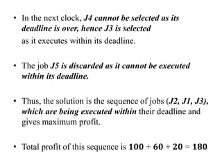
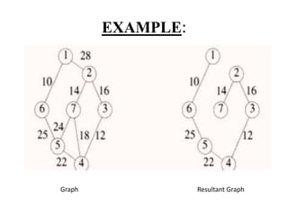
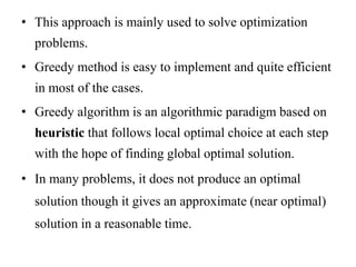
14. AlgorithmJS(d,j,n)
//d[i]≥1, 1 ≤ i ≤ n are the deadlines.
//The jobs are ordered such that p[1] ≥p[2] …… ≥p[n]
// j[i] is the ith job in the optimal solution, 1≤ i ≤ k
{
d[0]=j[0]=0; // Initialize
j[1]=1; // Include job 1 which is having highest profit
k=1; // no of jobs considered till now
for i=2 to n do
{ //Consider jobs in Descending order of p[i].
// Find position for i and check feasibility of insertion.
r=k;

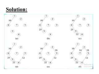
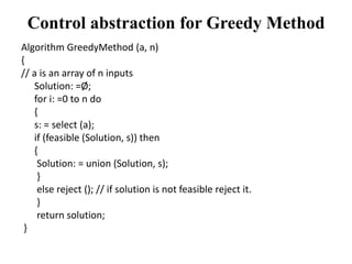
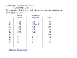
15. while( ( d[ j[r] ] > d[ i ] ) and ( d[ j[ r ] ] != r ) ) do
//checking present job with existing jobs in array and try to shift job towards
upwards in list
{
r = r-1;
}
if( d[ j[r] ] ≤ d[i] and d[ i ] > r )) then //job can be inserted or not
{
// Insert i into j[ ].
for q=k to (r+1) step -1 do // shift existing jobs downwards
{
j[q+1] = j[q];
}
j[r+1] :=i; // insert job in sequence
k:=k+1; // increase job count
} }
return k; }
Time taken by this algorithm is o(n2)

16. Assignment
• Let n=4 (p1…p4)=(20,15,10,5,1)
(d1…d4)=(2,2,1,3,3)

17. 0/1 knapsack problem
• The Greedy algorithm could be understood
very well with a well-known problem referred
to as Knapsack problem.
• Although the same problem could be solved by
employing other algorithmic approaches.
• Greedy approach solves Fractional Knapsack
problem reasonably in a good time.

18. • There are items i1, i2, ..., in each having
weight w1, w2, … wn and some benefit (value
or profit) associated with it p1, p2, ..., pn
• Our objective is to maximize the benefit or
profit such that the total weight inside the
knapsack is at most M, and we are also
allowed to take an item in fractional part.

19. • There are n items in the store
-weight of ith item 𝒘𝒊 > 𝟎
- Profit for ith item 𝒑𝒊 > 𝟎 and
• Capacity of the Knapsack is M.
• In this version of Knapsack problem, items can be broken
into smaller pieces, take fraction xi of ith item.
𝟎 ≤ 𝒙𝒊 ≤ 𝟏
• The ith item contributes the weight 𝒙𝒊*𝒘𝒊 to the total
weight in the knapsack and profit 𝒙𝒊*𝒑𝒊 to the total profit.
Hence, the objective of this algorithm is to
𝒎𝒂𝒙𝒊𝒎𝒊𝒛𝒆 Σn=1 to n (𝒙𝒊. 𝒑𝒊)

20. • subject to constraint,
Σn=1 to n(𝒙𝒊. 𝒘𝒊)≤ M
• It is clear that an optimal solution must fill the
knapsack exactly, otherwise we could add a fraction of
one of the remaining items and increase the overall
profit.
• Thus, an optimal solution can be obtained by
Σn=1 to n(𝒙𝒊. 𝒘𝒊)= M
• In this context, first we need to sort those items
according to the value of 𝒑𝒊/𝒘𝒊, so that (𝒑𝒊+𝟏)/(𝒘𝒊+𝟏)≤
𝒑𝒊/𝒘𝒊.
• Here, x is an array to store the fraction of items.

22. • Example 1:
Let us consider that the capacity of the
knapsack M = 𝟔𝟎 and the list of provided item
are shown in the following table:
ITEM A B C D
PROFIT 280 100 120 120
WEIGHT 40 10 20 24
RATIO (Pi/Wi)

23. • As the provided items are not sorted based on pi / wi. After sorting,
the items are as shown in the following table.
• After sorting all the items according to 𝒑𝒊/𝒘𝒊. First all of B is chosen
as weight of B is less than the capacity of the knapsack.
• Next, item A is chosen, as the available capacity of the knapsack is
greater than the weight of A.
• Now, C is chosen as the next item. However, the whole item cannot
be chosen as the remaining capacity of the knapsack is less than
the weight of C.
Hence, fraction of C (i.e. (60 − 50)/20) is chosen.
ITEM B A C D
PROFIT 100 280 120 120
WEIGHT 10 40 20 24
RATIO (Pi/Wi) 10 7 6 5

24. • Now, the capacity of the Knapsack is equal to the
selected items. Hence, no more item
can be selected.
• The total weight of the selected items is 𝟏𝟎 + 𝟒𝟎
+ 𝟐𝟎 ∗ (𝟏𝟎/𝟐𝟎) = 𝟔𝟎
• And the total profit is 𝟏𝟎𝟎 + 𝟐𝟖𝟎 + 𝟏𝟐𝟎 ∗ (𝟏𝟎/𝟐𝟎
) = 𝟑𝟖𝟎 + 𝟔𝟎 = 𝟒𝟒𝟎
• This is the optimal solution. We cannot gain more
profit selecting any different combination of
items.

25. Example 2: KANPSACK SIZE IS M=16
ITEM WEIGHT PROFIT
1 6 6
2 10 2
3 3 1
4 5 8
5 1 3
6 3 5

26. Minimum Cost Spanning Trees
• A spanning tree is a subset of Graph G, which
has all the vertices covered with minimum
possible number of edges.
• Hence, a spanning tree does not have cycles
and it cannot be disconnected.
-Note 1: Every connected and undirected
Graph G has at least one spanning tree.
-Note 2: A disconnected graph does not have
any spanning tree.

28. Kruskal’s Algorithm
Step 1 - Remove all loops and Parallel Edges.
Step 2 - Arrange all edges in their increasing
order of weight.
Step 3 - Add the edge which has the least
weight iff it does not form cycle.

31. • 1-6 ->10

33. Total min cost of spanning tree is 10+12+14+16+22+25=99

37. Time Complexity: O(ElogE) or O(ElogV). Sorting
of edges takes O(ELogE) time. After sorting, we
iterate through all edges and apply the find-union
algorithm. The find and union operations can take
at most O(LogV) time. So overall complexity is
O(ELogE + ELogV) time. The value of E can be at
most O(V2), so O(LogV) is O(LogE) the same.
Therefore, the overall time complexity is O(ElogE)
or O(ElogV)

49. Prim’s Algorithm
• Prim's algorithm treats the nodes as a single tree
and keeps on adding new nodes to the spanning
tree from the given graph.
- Step 1 - Remove all loops and parallel edges.
-Step 2 - Choose any arbitrary node as root node
with mincost.
- Step 3 - Check outgoing edges and select the one
with less cost.

50. EXAMPLE:
Graph Resultant Graph

57. Solution:

60. Kruskal’s vs Prim’s
• Prim’s algorithm initializes with a node, where as
Kruskal’s algorithm initiates with an edge.
• Prim’s algorithms span from one node to another
while Kruskal’s algorithm select the edges in a
way that the position of the edges is not based on
the last step.
• In prim’s algorithm , graph must be a connected
graph while the kruskal’s can function on
disconnected graphs too.
• Prim’s algorithm has Time complexity of O(V2),
and Kruskal’s Time Complexity is O(E log V)

61. Single source shortest path
(Dijkstra’s algorithm)
• For a given source node in the graph, the
algorithm finds the shortest path between that
node and other nodes.
• It also used for finding the shortest paths from
a single node to a single destination node by
stopping the algorithm once the shortest path
to the destination node has been determined.

68. Example: