CS501: DATABASE AND
DATA MINING
Classification and Prediction1
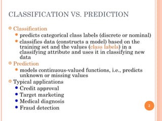
CLASSIFICATION VS. PREDICTION
 Classification
predicts categorical class labels (discrete or nominal)
classifies data (constructs a model) based on the
training set and the values (class labels) in a
classifying attribute and uses it in classifying new
data
 Prediction
models continuous-valued functions, i.e., predicts
unknown or missing values
 Typical applications
Credit approval
Target marketing
Medical diagnosis
Fraud detection
2
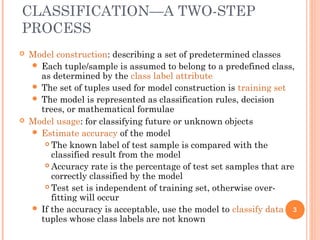
CLASSIFICATION—A TWO-STEP
PROCESS
 Model construction: describing a set of predetermined classes
 Each tuple/sample is assumed to belong to a predefined class,
as determined by the class label attribute
 The set of tuples used for model construction is training set
 The model is represented as classification rules, decision
trees, or mathematical formulae
 Model usage: for classifying future or unknown objects
 Estimate accuracy of the model
 The known label of test sample is compared with the
classified result from the model
 Accuracy rate is the percentage of test set samples that are
correctly classified by the model
 Test set is independent of training set, otherwise over-
fitting will occur
 If the accuracy is acceptable, use the model to classify data
tuples whose class labels are not known
3
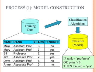
PROCESS (1): MODEL CONSTRUCTION
4
Training
Data
NAME RANK YEARS TENURED
Mike Assistant Prof 3 no
Mary Assistant Prof 7 yes
Bill Professor 2 yes
Jim Associate Prof 7 yes
Dave Assistant Prof 6 no
Anne Associate Prof 3 no
Classification
Algorithms
IF rank = ‘professor’
OR years > 6
THEN tenured = ‘yes’
Classifier
(Model)
PROCESS (2): USING THE MODEL IN
PREDICTION
5
Classifier
Testing
Data
NAME RANK YEARS TENURED
Tom Assistant Prof 2 no
Merlisa Associate Prof 7 no
George Professor 5 yes
Joseph Assistant Prof 7 yes
Unseen Data
(Jeff, Professor, 4)
Tenured?
SUPERVISED VS. UNSUPERVISED
LEARNING
 Supervised learning (classification)
Supervision: The training data (observations,
measurements, etc.) are accompanied by labels
indicating the class of the observations
New data is classified based on the training set
 Unsupervised learning (clustering)
The class labels of training data is unknown
Given a set of measurements, observations, etc.
with the aim of establishing the existence of classes
or clusters in the data
6
ISSUES: DATA PREPARATION
 Data cleaning
Preprocess data in order to reduce noise and handle
missing values
 Relevance analysis (feature selection)
Remove the irrelevant or redundant attributes
 Data transformation
Generalize and/or normalize data
7
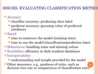
ISSUES: EVALUATING CLASSIFICATION METHOD
 Accuracy
classifier accuracy: predicting class label
predictor accuracy: guessing value of predicted
attributes
 Speed
time to construct the model (training time)
time to use the model (classification/prediction time)
 Robustness: handling noise and missing values
 Scalability: efficiency in disk-resident databases
 Interpretability
understanding and insight provided by the model
 Other measures, e.g., goodness of rules, such as
decision tree size or compactness of classification rules
8
DECISION TREE INDUCTION: TRAINING
DATASET
age income student credit_rating buys_computer
<=30 high no fair no
<=30 high no excellent no
31…40 high no fair yes
>40 medium no fair yes
>40 low yes fair yes
>40 low yes excellent no
31…40 low yes excellent yes
<=30 medium no fair no
<=30 low yes fair yes
>40 medium yes fair yes
<=30 medium yes excellent yes
31…40 medium no excellent yes
31…40 high yes fair yes
>40 medium no excellent no
9
OUTPUT: A DECISION TREE FOR
“BUYS_COMPUTER”
10
age?
overcast
student? credit rating?
<=30 >40
no yes yes
yes
31..40
no
fairexcellentyesno
ALGORITHM FOR DECISION TREE
INDUCTION
 Basic algorithm (a greedy algorithm)
 Tree is constructed in a top-down recursive divide-and-conquer
manner
 At start, all the training examples are at the root
 Attributes are categorical (if continuous-valued, they are
discretized in advance)
 Examples are partitioned recursively based on selected
attributes
 Test attributes are selected on the basis of a heuristic or
statistical measure (e.g., information gain)
 Conditions for stopping partitioning
 All samples for a given node belong to the same class
 There are no remaining attributes for further partitioning –
majority voting is employed for classifying the leaf
 There are no samples left
11
12
Attribute Selection Measure:
Information Gain (ID3/C4.5)
 Select the attribute with the highest information gain
 Let pi be the probability that an arbitrary tuple in D belongs
to class Ci, estimated by |Ci, D|/|D|
 Expected information (entropy) needed to classify a tuple
in D:
 Information needed (after using A to split D into v
partitions) to classify D:
 Information gained by branching on attribute A
)(log)( 2
1
i
m
i
i ppDInfo ∑=
−=
)(
||
||
)(
1
j
v
j
j
A DInfo
D
D
DInfo ×= ∑=
(D)InfoInfo(D)Gain(A) A−=
ATTRIBUTE SELECTION: INFORMATION
GAIN
13
 Class P: buys_computer = “yes”
 Class N: buys_computer = “no”
means “age <=30” has 5
out of 14 samples, with 2 yes’es
and 3 no’s. Hence
age pi ni I(pi, ni)
<=30 2 3 0.971
31…40 4 0 0
>40 3 2 0.971
694.0)2,3(
14
5
)0,4(
14
4
)3,2(
14
5
)(
=+
+=
I
IIDInfoage
048.0)_(
151.0)(
029.0)(
=
=
=
ratingcreditGain
studentGain
incomeGain
246.0)()()( =−= DInfoDInfoageGain age
age income student credit_rating buys_computer
<=30 high no fair no
<=30 high no excellent no
31…40 high no fair yes
>40 medium no fair yes
>40 low yes fair yes
>40 low yes excellent no
31…40 low yes excellent yes
<=30 medium no fair no
<=30 low yes fair yes
>40 medium yes fair yes
<=30 medium yes excellent yes
31…40 medium no excellent yes
31…40 high yes fair yes
>40 medium no excellent no
)3,2(
14
5
I
940.0)
14
5
(log
14
5
)
14
9
(log
14
9
)5,9()( 22 =−−== IDInfo
Similarly,
COMPUTING INFORMATION-GAIN FOR
CONTINUOUS-VALUE ATTRIBUTES
 Let attribute A be a continuous-valued attribute
 Must determine the best split point for A
Sort the value A in increasing order
Typically, the midpoint between each pair of adjacent
values is considered as a possible split point
 (ai+ai+1)/2 is the midpoint between the values of ai and ai+1
The point with the minimum expected information
requirement for A is selected as the split-point for A
 Split:
D1 is the set of tuples in D satisfying A ≤ split-point,
and D2 is the set of tuples in D satisfying A > split-
14
GAIN RATIO FOR ATTRIBUTE SELECTION
(C4.5)
 Information gain measure is biased towards attributes
with a large number of values
 C4.5 (a successor of ID3) uses gain ratio to overcome the
problem (normalization to information gain)
GainRatio(A) = Gain(A)/SplitInfo(A)
 Ex.
gain_ratio(income) = 0.029/0.926 = 0.031
 The attribute with the maximum gain ratio is selected
as the splitting attribute
)
||
||
(log
||
||
)( 2
1 D
D
D
D
DSplitInfo
j
v
j
j
A ×−= ∑=
926.0)
14
4
(log
14
4
)
14
6
(log
14
6
)
14
4
(log
14
4
)( 222 =×−×−×−=DSplitInfoincome
15
GINI INDEX (CART, IBM
INTELLIGENTMINER)
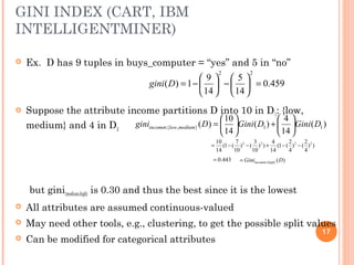
 If a data set D contains examples from n classes, gini index, gini(D)
is defined as
where pj is the relative frequency of class j in D
 If a data set D is split on A into two subsets D1 and D2, the gini
index gini(D) is defined as
 Reduction in Impurity:
 The attribute provides the smallest ginisplit(D) (or the largest
reduction in impurity) is chosen to split the node (need to enumerate
all the possible splitting points for each attribute)
)()()( DginiDginiAgini A
−=∆
16
∑
=
−=
n
j
p jDgini
1
21)(
)(
||
||
)(
||
||
)( 2
2
1
1
Dgini
D
D
Dgini
D
D
DginiA
+=
GINI INDEX (CART, IBM
INTELLIGENTMINER)
 Ex. D has 9 tuples in buys_computer = “yes” and 5 in “no”
 Suppose the attribute income partitions D into 10 in D1: {low,
medium} and 4 in D2
but gini{medium,high} is 0.30 and thus the best since it is the lowest
 All attributes are assumed continuous-valued
 May need other tools, e.g., clustering, to get the possible split values
 Can be modified for categorical attributes
459.0
14
5
14
9
1)(
22
=





−





−=Dgini
17
)(
14
4
)(
14
10
)( 11},{ DGiniDGiniDgini mediumlowincome 





+





=∈
))
4
2
()
4
2
(1(
14
4
))
10
3
()
10
7
(1(
14
10 2222
−−+−−=
443.0= )(}{ DGini highincome∈=
COMPARING ATTRIBUTE SELECTION
MEASURES
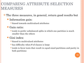
 The three measures, in general, return good results but
Information gain:
 biased towards multivalued attributes
Gain ratio:
 tends to prefer unbalanced splits in which one partition is much
smaller than the others
Gini index:
 biased to multivalued attributes
 has difficulty when # of classes is large
 tends to favor tests that result in equal-sized partitions and purity in
both partitions
18
OVERFITTING AND TREE PRUNING
 Overfitting: An induced tree may overfit the training
data
 Too many branches, some may reflect anomalies due to noise or
outliers
 Poor accuracy for unseen samples
 Two approaches to avoid overfitting
 Prepruning: Halt tree construction early—do not split a node if
this would result in the goodness measure falling below a
threshold
 Difficult to choose an appropriate threshold
 Postpruning: Remove branches from a “fully grown” tree—get a
sequence of progressively pruned trees
 Use a set of data different from the training data to decide
which is the “best pruned tree”
19
ENHANCEMENTS TO BASIC DECISION TREE
INDUCTION
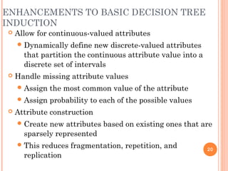
 Allow for continuous-valued attributes
Dynamically define new discrete-valued attributes
that partition the continuous attribute value into a
discrete set of intervals
 Handle missing attribute values
Assign the most common value of the attribute
Assign probability to each of the possible values
 Attribute construction
Create new attributes based on existing ones that are
sparsely represented
This reduces fragmentation, repetition, and
replication
20
USING IF-THEN RULES FOR
CLASSIFICATION
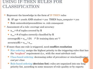
 Represent the knowledge in the form of IF-THEN rules
R: IF age = youth AND student = yes THEN buys_computer = yes
 Rule antecedent/precondition vs. rule consequent
 Assessment of a rule: coverage and accuracy
 ncovers = # of tuples covered by R
 ncorrect = # of tuples correctly classified by R
coverage(R) = ncovers /|D| /* D: training data set */
accuracy(R) = ncorrect / ncovers
 If more than one rule is triggered, need conflict resolution
 Size ordering: assign the highest priority to the triggering rules that has
the “toughest” requirement (i.e., with the most attribute test)
 Class-based ordering: decreasing order of prevalence or misclassification
cost per class
 Rule-based ordering (decision list): rules are organized into one long
priority list, according to some measure of rule quality or by experts
21
RULE EXTRACTION FROM A DECISION
TREE
 Example: Rule extraction from our buys_computer decision-tree
IF age = young AND student = no THEN buys_computer = no
IF age = young AND student = yes THEN buys_computer = yes
IF age = mid-age THEN buys_computer = yes
IF age = old AND credit_rating = excellent THEN buys_computer = yes
IF age = young AND credit_rating = fair THEN buys_computer = no
22
age?
student? credit rating?
<=30 >40
no yes yes
yes
31..40
no
fairexcellentyesno
 Rules are easier to understand than large trees
 One rule is created for each path from the root to
a leaf
 Each attribute-value pair along a path forms a
conjunction: the leaf holds the class prediction
 Rules are mutually exclusive and exhaustive
RULE EXTRACTION FROM THE
TRAINING DATA
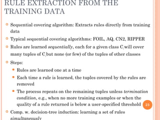
 Sequential covering algorithm: Extracts rules directly from training
data
 Typical sequential covering algorithms: FOIL, AQ, CN2, RIPPER
 Rules are learned sequentially, each for a given class Ci will cover
many tuples of Ci but none (or few) of the tuples of other classes
 Steps:
 Rules are learned one at a time
 Each time a rule is learned, the tuples covered by the rules are
removed
 The process repeats on the remaining tuples unless termination
condition, e.g., when no more training examples or when the
quality of a rule returned is below a user-specified threshold
 Comp. w. decision-tree induction: learning a set of rules
simultaneously
23
HOW TO LEARN-ONE-RULE?
 Start with the most general rule possible: condition = empty
 Adding new attributes by adopting a greedy depth-first strategy
 Picks the one that most improves the rule quality
 Rule-Quality measures: consider both coverage and accuracy
 Foil-gain (in FOIL & RIPPER): assesses info_gain by extending
condition
It favors rules that have high accuracy and cover many positive tuples
 Rule pruning based on an independent set of test tuples
Pos/neg are # of positive/negative tuples covered by R.
If FOIL_Prune is higher for the pruned version of R, prune R
)log
''
'
(log'_ 22
negpos
pos
negpos
pos
posGainFOIL
+
−
+
×=
negpos
negpos
RPruneFOIL
+
−
=)(_
24
WHAT IS PREDICTION?
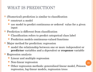
 (Numerical) prediction is similar to classification
 construct a model
 use model to predict continuous or ordered value for a given
input
 Prediction is different from classification
 Classification refers to predict categorical class label
 Prediction models continuous-valued functions
 Major method for prediction: regression
 model the relationship between one or more independent or
predictor variables and a dependent or response variable
 Regression analysis
 Linear and multiple regression
 Non-linear regression
 Other regression methods: generalized linear model, Poisson
regression, log-linear models, regression trees
25
LINEAR REGRESSION
 Linear regression: involves a response variable y and a single
predictor variable x
y = w0 + w1 x
where w0 (y-intercept) and w1 (slope) are regression coefficients
 Method of least squares: estimates the best-fitting straight line
 Multiple linear regression: involves more than one predictor
variable
 Training data is of the form (X1, y1), (X2, y2),…, (X|D|, y|D|)
 Ex. For 2-D data, we may have: y = w0 + w1 x1+ w2 x2
 Solvable by extension of least square method or using SAS, S-
∑
∑
=
=
−
−−
= ||
1
2
||
1
)(
))((
1 D
i
i
D
i
ii
xx
yyxx
w xwyw
10
−=
26
NONLINEAR REGRESSION
 Some nonlinear models can be modeled by a polynomial
function
 A polynomial regression model can be transformed into
linear regression model. For example,
y = w0 + w1 x + w2 x2
+ w3 x3
convertible to linear with new variables: x2 = x2
, x3= x3
y = w0 + w1 x + w2 x2 + w3 x3
 Other functions, such as power function, can also be
transformed to linear model
 Some models are intractable nonlinear (e.g., sum of
exponential terms)
possible to obtain least square estimates through
extensive calculation on more complex formulae
27
CLASSIFIER ACCURACY
MEASURES
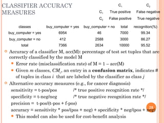
 Accuracy of a classifier M, acc(M): percentage of test set tuples that are
correctly classified by the model M
 Error rate (misclassification rate) of M = 1 – acc(M)
 Given m classes, CMi,j, an entry in a confusion matrix, indicates #
of tuples in class i that are labeled by the classifier as class j
 Alternative accuracy measures (e.g., for cancer diagnosis)
sensitivity = t-pos/pos /* true positive recognition rate */
specificity = t-neg/neg /* true negative recognition rate */
precision = t-pos/(t-pos + f-pos)
accuracy = sensitivity * pos/(pos + neg) + specificity * neg/(pos + neg)
 This model can also be used for cost-benefit analysis
C1 C2
C1 True positive False negative
C2 False positive True negative
classes buy_computer = yes buy_computer = no total recognition(%)
buy_computer = yes 6954 46 7000 99.34
buy_computer = no 412 2588 3000 86.27
total 7366 2634 10000 95.52
28
EVALUATING THE ACCURACY OF A
CLASSIFIER OR PREDICTOR (I)
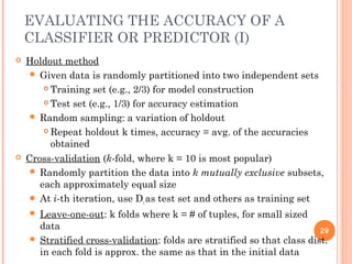
 Holdout method
 Given data is randomly partitioned into two independent sets
 Training set (e.g., 2/3) for model construction
 Test set (e.g., 1/3) for accuracy estimation
 Random sampling: a variation of holdout
 Repeat holdout k times, accuracy = avg. of the accuracies
obtained
 Cross-validation (k-fold, where k = 10 is most popular)
 Randomly partition the data into k mutually exclusive subsets,
each approximately equal size
 At i-th iteration, use Di as test set and others as training set
 Leave-one-out: k folds where k = # of tuples, for small sized
data
 Stratified cross-validation: folds are stratified so that class dist.
in each fold is approx. the same as that in the initial data
29
EVALUATING THE ACCURACY OF A
CLASSIFIER OR PREDICTOR (II)
 Bootstrap
 Works well with small data sets
 Samples the given training tuples uniformly with replacement
 i.e., each time a tuple is selected, it is equally likely to be
selected again and re-added to the training set
 Several boostrap methods, and a common one is .632 boostrap
 Suppose we are given a data set of d tuples. The data set is sampled d
times, with replacement, resulting in a training set of d samples. The
data tuples that did not make it into the training set end up forming the
test set. About 63.2% of the original data will end up in the bootstrap,
and the remaining 36.8% will form the test set (since (1 – 1/d)d
≈ e-1
=
0.368)
 Repeat the sampling procedue k times, overall accuracy of the
model:
))(368.0)(632.0()( _
1
_ settraini
k
i
settesti MaccMaccMacc ×+×= ∑=
30

Cs501 classification prediction

  • 1.
    CS501: DATABASE AND DATAMINING Classification and Prediction1
  • 2.
    CLASSIFICATION VS. PREDICTION Classification predicts categorical class labels (discrete or nominal) classifies data (constructs a model) based on the training set and the values (class labels) in a classifying attribute and uses it in classifying new data  Prediction models continuous-valued functions, i.e., predicts unknown or missing values  Typical applications Credit approval Target marketing Medical diagnosis Fraud detection 2
  • 3.
    CLASSIFICATION—A TWO-STEP PROCESS  Modelconstruction: describing a set of predetermined classes  Each tuple/sample is assumed to belong to a predefined class, as determined by the class label attribute  The set of tuples used for model construction is training set  The model is represented as classification rules, decision trees, or mathematical formulae  Model usage: for classifying future or unknown objects  Estimate accuracy of the model  The known label of test sample is compared with the classified result from the model  Accuracy rate is the percentage of test set samples that are correctly classified by the model  Test set is independent of training set, otherwise over- fitting will occur  If the accuracy is acceptable, use the model to classify data tuples whose class labels are not known 3
  • 4.
    PROCESS (1): MODELCONSTRUCTION 4 Training Data NAME RANK YEARS TENURED Mike Assistant Prof 3 no Mary Assistant Prof 7 yes Bill Professor 2 yes Jim Associate Prof 7 yes Dave Assistant Prof 6 no Anne Associate Prof 3 no Classification Algorithms IF rank = ‘professor’ OR years > 6 THEN tenured = ‘yes’ Classifier (Model)
  • 5.
    PROCESS (2): USINGTHE MODEL IN PREDICTION 5 Classifier Testing Data NAME RANK YEARS TENURED Tom Assistant Prof 2 no Merlisa Associate Prof 7 no George Professor 5 yes Joseph Assistant Prof 7 yes Unseen Data (Jeff, Professor, 4) Tenured?
  • 6.
    SUPERVISED VS. UNSUPERVISED LEARNING Supervised learning (classification) Supervision: The training data (observations, measurements, etc.) are accompanied by labels indicating the class of the observations New data is classified based on the training set  Unsupervised learning (clustering) The class labels of training data is unknown Given a set of measurements, observations, etc. with the aim of establishing the existence of classes or clusters in the data 6
  • 7.
    ISSUES: DATA PREPARATION Data cleaning Preprocess data in order to reduce noise and handle missing values  Relevance analysis (feature selection) Remove the irrelevant or redundant attributes  Data transformation Generalize and/or normalize data 7
  • 8.
    ISSUES: EVALUATING CLASSIFICATIONMETHOD  Accuracy classifier accuracy: predicting class label predictor accuracy: guessing value of predicted attributes  Speed time to construct the model (training time) time to use the model (classification/prediction time)  Robustness: handling noise and missing values  Scalability: efficiency in disk-resident databases  Interpretability understanding and insight provided by the model  Other measures, e.g., goodness of rules, such as decision tree size or compactness of classification rules 8
  • 9.
    DECISION TREE INDUCTION:TRAINING DATASET age income student credit_rating buys_computer <=30 high no fair no <=30 high no excellent no 31…40 high no fair yes >40 medium no fair yes >40 low yes fair yes >40 low yes excellent no 31…40 low yes excellent yes <=30 medium no fair no <=30 low yes fair yes >40 medium yes fair yes <=30 medium yes excellent yes 31…40 medium no excellent yes 31…40 high yes fair yes >40 medium no excellent no 9
  • 10.
    OUTPUT: A DECISIONTREE FOR “BUYS_COMPUTER” 10 age? overcast student? credit rating? <=30 >40 no yes yes yes 31..40 no fairexcellentyesno
  • 11.
    ALGORITHM FOR DECISIONTREE INDUCTION  Basic algorithm (a greedy algorithm)  Tree is constructed in a top-down recursive divide-and-conquer manner  At start, all the training examples are at the root  Attributes are categorical (if continuous-valued, they are discretized in advance)  Examples are partitioned recursively based on selected attributes  Test attributes are selected on the basis of a heuristic or statistical measure (e.g., information gain)  Conditions for stopping partitioning  All samples for a given node belong to the same class  There are no remaining attributes for further partitioning – majority voting is employed for classifying the leaf  There are no samples left 11
  • 12.
    12 Attribute Selection Measure: InformationGain (ID3/C4.5)  Select the attribute with the highest information gain  Let pi be the probability that an arbitrary tuple in D belongs to class Ci, estimated by |Ci, D|/|D|  Expected information (entropy) needed to classify a tuple in D:  Information needed (after using A to split D into v partitions) to classify D:  Information gained by branching on attribute A )(log)( 2 1 i m i i ppDInfo ∑= −= )( || || )( 1 j v j j A DInfo D D DInfo ×= ∑= (D)InfoInfo(D)Gain(A) A−=
  • 13.
    ATTRIBUTE SELECTION: INFORMATION GAIN 13 Class P: buys_computer = “yes”  Class N: buys_computer = “no” means “age <=30” has 5 out of 14 samples, with 2 yes’es and 3 no’s. Hence age pi ni I(pi, ni) <=30 2 3 0.971 31…40 4 0 0 >40 3 2 0.971 694.0)2,3( 14 5 )0,4( 14 4 )3,2( 14 5 )( =+ += I IIDInfoage 048.0)_( 151.0)( 029.0)( = = = ratingcreditGain studentGain incomeGain 246.0)()()( =−= DInfoDInfoageGain age age income student credit_rating buys_computer <=30 high no fair no <=30 high no excellent no 31…40 high no fair yes >40 medium no fair yes >40 low yes fair yes >40 low yes excellent no 31…40 low yes excellent yes <=30 medium no fair no <=30 low yes fair yes >40 medium yes fair yes <=30 medium yes excellent yes 31…40 medium no excellent yes 31…40 high yes fair yes >40 medium no excellent no )3,2( 14 5 I 940.0) 14 5 (log 14 5 ) 14 9 (log 14 9 )5,9()( 22 =−−== IDInfo Similarly,
  • 14.
    COMPUTING INFORMATION-GAIN FOR CONTINUOUS-VALUEATTRIBUTES  Let attribute A be a continuous-valued attribute  Must determine the best split point for A Sort the value A in increasing order Typically, the midpoint between each pair of adjacent values is considered as a possible split point  (ai+ai+1)/2 is the midpoint between the values of ai and ai+1 The point with the minimum expected information requirement for A is selected as the split-point for A  Split: D1 is the set of tuples in D satisfying A ≤ split-point, and D2 is the set of tuples in D satisfying A > split- 14
  • 15.
    GAIN RATIO FORATTRIBUTE SELECTION (C4.5)  Information gain measure is biased towards attributes with a large number of values  C4.5 (a successor of ID3) uses gain ratio to overcome the problem (normalization to information gain) GainRatio(A) = Gain(A)/SplitInfo(A)  Ex. gain_ratio(income) = 0.029/0.926 = 0.031  The attribute with the maximum gain ratio is selected as the splitting attribute ) || || (log || || )( 2 1 D D D D DSplitInfo j v j j A ×−= ∑= 926.0) 14 4 (log 14 4 ) 14 6 (log 14 6 ) 14 4 (log 14 4 )( 222 =×−×−×−=DSplitInfoincome 15
  • 16.
    GINI INDEX (CART,IBM INTELLIGENTMINER)  If a data set D contains examples from n classes, gini index, gini(D) is defined as where pj is the relative frequency of class j in D  If a data set D is split on A into two subsets D1 and D2, the gini index gini(D) is defined as  Reduction in Impurity:  The attribute provides the smallest ginisplit(D) (or the largest reduction in impurity) is chosen to split the node (need to enumerate all the possible splitting points for each attribute) )()()( DginiDginiAgini A −=∆ 16 ∑ = −= n j p jDgini 1 21)( )( || || )( || || )( 2 2 1 1 Dgini D D Dgini D D DginiA +=
  • 17.
    GINI INDEX (CART,IBM INTELLIGENTMINER)  Ex. D has 9 tuples in buys_computer = “yes” and 5 in “no”  Suppose the attribute income partitions D into 10 in D1: {low, medium} and 4 in D2 but gini{medium,high} is 0.30 and thus the best since it is the lowest  All attributes are assumed continuous-valued  May need other tools, e.g., clustering, to get the possible split values  Can be modified for categorical attributes 459.0 14 5 14 9 1)( 22 =      −      −=Dgini 17 )( 14 4 )( 14 10 )( 11},{ DGiniDGiniDgini mediumlowincome       +      =∈ )) 4 2 () 4 2 (1( 14 4 )) 10 3 () 10 7 (1( 14 10 2222 −−+−−= 443.0= )(}{ DGini highincome∈=
  • 18.
    COMPARING ATTRIBUTE SELECTION MEASURES The three measures, in general, return good results but Information gain:  biased towards multivalued attributes Gain ratio:  tends to prefer unbalanced splits in which one partition is much smaller than the others Gini index:  biased to multivalued attributes  has difficulty when # of classes is large  tends to favor tests that result in equal-sized partitions and purity in both partitions 18
  • 19.
    OVERFITTING AND TREEPRUNING  Overfitting: An induced tree may overfit the training data  Too many branches, some may reflect anomalies due to noise or outliers  Poor accuracy for unseen samples  Two approaches to avoid overfitting  Prepruning: Halt tree construction early—do not split a node if this would result in the goodness measure falling below a threshold  Difficult to choose an appropriate threshold  Postpruning: Remove branches from a “fully grown” tree—get a sequence of progressively pruned trees  Use a set of data different from the training data to decide which is the “best pruned tree” 19
  • 20.
    ENHANCEMENTS TO BASICDECISION TREE INDUCTION  Allow for continuous-valued attributes Dynamically define new discrete-valued attributes that partition the continuous attribute value into a discrete set of intervals  Handle missing attribute values Assign the most common value of the attribute Assign probability to each of the possible values  Attribute construction Create new attributes based on existing ones that are sparsely represented This reduces fragmentation, repetition, and replication 20
  • 21.
    USING IF-THEN RULESFOR CLASSIFICATION  Represent the knowledge in the form of IF-THEN rules R: IF age = youth AND student = yes THEN buys_computer = yes  Rule antecedent/precondition vs. rule consequent  Assessment of a rule: coverage and accuracy  ncovers = # of tuples covered by R  ncorrect = # of tuples correctly classified by R coverage(R) = ncovers /|D| /* D: training data set */ accuracy(R) = ncorrect / ncovers  If more than one rule is triggered, need conflict resolution  Size ordering: assign the highest priority to the triggering rules that has the “toughest” requirement (i.e., with the most attribute test)  Class-based ordering: decreasing order of prevalence or misclassification cost per class  Rule-based ordering (decision list): rules are organized into one long priority list, according to some measure of rule quality or by experts 21
  • 22.
    RULE EXTRACTION FROMA DECISION TREE  Example: Rule extraction from our buys_computer decision-tree IF age = young AND student = no THEN buys_computer = no IF age = young AND student = yes THEN buys_computer = yes IF age = mid-age THEN buys_computer = yes IF age = old AND credit_rating = excellent THEN buys_computer = yes IF age = young AND credit_rating = fair THEN buys_computer = no 22 age? student? credit rating? <=30 >40 no yes yes yes 31..40 no fairexcellentyesno  Rules are easier to understand than large trees  One rule is created for each path from the root to a leaf  Each attribute-value pair along a path forms a conjunction: the leaf holds the class prediction  Rules are mutually exclusive and exhaustive
  • 23.
    RULE EXTRACTION FROMTHE TRAINING DATA  Sequential covering algorithm: Extracts rules directly from training data  Typical sequential covering algorithms: FOIL, AQ, CN2, RIPPER  Rules are learned sequentially, each for a given class Ci will cover many tuples of Ci but none (or few) of the tuples of other classes  Steps:  Rules are learned one at a time  Each time a rule is learned, the tuples covered by the rules are removed  The process repeats on the remaining tuples unless termination condition, e.g., when no more training examples or when the quality of a rule returned is below a user-specified threshold  Comp. w. decision-tree induction: learning a set of rules simultaneously 23
  • 24.
    HOW TO LEARN-ONE-RULE? Start with the most general rule possible: condition = empty  Adding new attributes by adopting a greedy depth-first strategy  Picks the one that most improves the rule quality  Rule-Quality measures: consider both coverage and accuracy  Foil-gain (in FOIL & RIPPER): assesses info_gain by extending condition It favors rules that have high accuracy and cover many positive tuples  Rule pruning based on an independent set of test tuples Pos/neg are # of positive/negative tuples covered by R. If FOIL_Prune is higher for the pruned version of R, prune R )log '' ' (log'_ 22 negpos pos negpos pos posGainFOIL + − + ×= negpos negpos RPruneFOIL + − =)(_ 24
  • 25.
    WHAT IS PREDICTION? (Numerical) prediction is similar to classification  construct a model  use model to predict continuous or ordered value for a given input  Prediction is different from classification  Classification refers to predict categorical class label  Prediction models continuous-valued functions  Major method for prediction: regression  model the relationship between one or more independent or predictor variables and a dependent or response variable  Regression analysis  Linear and multiple regression  Non-linear regression  Other regression methods: generalized linear model, Poisson regression, log-linear models, regression trees 25
  • 26.
    LINEAR REGRESSION  Linearregression: involves a response variable y and a single predictor variable x y = w0 + w1 x where w0 (y-intercept) and w1 (slope) are regression coefficients  Method of least squares: estimates the best-fitting straight line  Multiple linear regression: involves more than one predictor variable  Training data is of the form (X1, y1), (X2, y2),…, (X|D|, y|D|)  Ex. For 2-D data, we may have: y = w0 + w1 x1+ w2 x2  Solvable by extension of least square method or using SAS, S- ∑ ∑ = = − −− = || 1 2 || 1 )( ))(( 1 D i i D i ii xx yyxx w xwyw 10 −= 26
  • 27.
    NONLINEAR REGRESSION  Somenonlinear models can be modeled by a polynomial function  A polynomial regression model can be transformed into linear regression model. For example, y = w0 + w1 x + w2 x2 + w3 x3 convertible to linear with new variables: x2 = x2 , x3= x3 y = w0 + w1 x + w2 x2 + w3 x3  Other functions, such as power function, can also be transformed to linear model  Some models are intractable nonlinear (e.g., sum of exponential terms) possible to obtain least square estimates through extensive calculation on more complex formulae 27
  • 28.
    CLASSIFIER ACCURACY MEASURES  Accuracyof a classifier M, acc(M): percentage of test set tuples that are correctly classified by the model M  Error rate (misclassification rate) of M = 1 – acc(M)  Given m classes, CMi,j, an entry in a confusion matrix, indicates # of tuples in class i that are labeled by the classifier as class j  Alternative accuracy measures (e.g., for cancer diagnosis) sensitivity = t-pos/pos /* true positive recognition rate */ specificity = t-neg/neg /* true negative recognition rate */ precision = t-pos/(t-pos + f-pos) accuracy = sensitivity * pos/(pos + neg) + specificity * neg/(pos + neg)  This model can also be used for cost-benefit analysis C1 C2 C1 True positive False negative C2 False positive True negative classes buy_computer = yes buy_computer = no total recognition(%) buy_computer = yes 6954 46 7000 99.34 buy_computer = no 412 2588 3000 86.27 total 7366 2634 10000 95.52 28
  • 29.
    EVALUATING THE ACCURACYOF A CLASSIFIER OR PREDICTOR (I)  Holdout method  Given data is randomly partitioned into two independent sets  Training set (e.g., 2/3) for model construction  Test set (e.g., 1/3) for accuracy estimation  Random sampling: a variation of holdout  Repeat holdout k times, accuracy = avg. of the accuracies obtained  Cross-validation (k-fold, where k = 10 is most popular)  Randomly partition the data into k mutually exclusive subsets, each approximately equal size  At i-th iteration, use Di as test set and others as training set  Leave-one-out: k folds where k = # of tuples, for small sized data  Stratified cross-validation: folds are stratified so that class dist. in each fold is approx. the same as that in the initial data 29
  • 30.
    EVALUATING THE ACCURACYOF A CLASSIFIER OR PREDICTOR (II)  Bootstrap  Works well with small data sets  Samples the given training tuples uniformly with replacement  i.e., each time a tuple is selected, it is equally likely to be selected again and re-added to the training set  Several boostrap methods, and a common one is .632 boostrap  Suppose we are given a data set of d tuples. The data set is sampled d times, with replacement, resulting in a training set of d samples. The data tuples that did not make it into the training set end up forming the test set. About 63.2% of the original data will end up in the bootstrap, and the remaining 36.8% will form the test set (since (1 – 1/d)d ≈ e-1 = 0.368)  Repeat the sampling procedue k times, overall accuracy of the model: ))(368.0)(632.0()( _ 1 _ settraini k i settesti MaccMaccMacc ×+×= ∑= 30

Editor's Notes

  • #13 I : the expected information needed to classify a given sample E (entropy) : expected information based on the partitioning into subsets by A