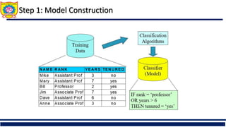
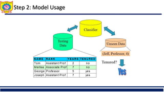
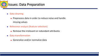
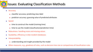
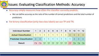
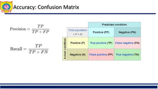
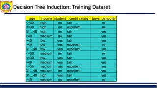
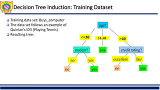
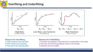
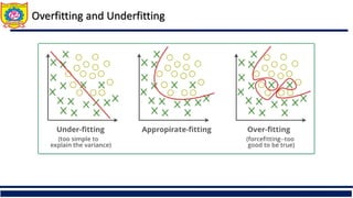
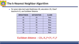
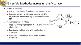
SlideShare a Scribd company logo
1 of 56
Download to read offline
Sanjivani Rural Education Society’s
Sanjivani College of Engineering, Kopargaon-423 603
(An Autonomous Institute, Affiliated to Savitribai Phule Pune University, Pune)
NACC ‘A’ Grade Accredited, ISO 9001:2015 Certified
Department of Computer Engineering
(NBA Accredited)
Prof. S. A. Shivarkar
Assistant Professor
Contact No.8275032712
Email- shivarkarsandipcomp@sanjivani.org.in
Subject- Data Mining and Warehousing (CO314)
Unit –VI: Classification
Content
 Introduction, classification requirements, methods of supervised learning
 Decision trees- attribute selection measures (info gain, Gini ratio, Gini
index), scalable decision tree techniques, rule extraction from decision tree,
Naïve bayesian Classification, Rule based classification
 Associative Classification, Lazy Learners-k-Nearest- Multiclass Classification,
Metrics for Evaluating Classifier Evaluating the Accuracy of a Classifier
 Regression, Introduction to Ensemble Methods.
Supervised vs. Unsupervised Learning
 Supervised learning (classification)
 Supervision: The training data (observations, measurements, etc.) are
accompanied by labels indicating the class of the observations
 New data is classified based on the training set
 Unsupervised learning (clustering)
 The class labels of training data is unknown
 Given a set of measurements, observations, etc. with the aim of
establishing the existence of classes or clusters in the data
Prediction Problems: Classification vs. Numeric Prediction
 Classification
 predicts categorical class labels (discrete or nominal)
 classifies data (constructs a model) based on the training set and the
values (class labels) in a classifying attribute and uses it in classifying new
data
 Numeric Prediction
 models continuous-valued functions, i.e., predicts unknown or missing
values
 Typical applications
 Credit/loan approval:
 Medical diagnosis: if a tumor is cancerous or benign
 Fraud detection: if a transaction is fraudulent
 Web page categorization: which category it is
Classification—A Two-Step Process
 Model construction: describing a set of predetermined classes
 Each tuple/sample is assumed to belong to a predefined class, as determined by the class
label attribute
 The set of tuples used for model construction is training set
 The model is represented as classification rules, decision trees, or mathematical formulae
 Model usage: for classifying future or unknown objects
 Estimate accuracy of the model
 The known label of test sample is compared with the classified result from the model
 Accuracy rate is the percentage of test set samples that are correctly classified by the
model
 Test set is independent of training set (otherwise overfitting)
 If the accuracy is acceptable, use the model to classify new data
 Note: If the test set is used to select models, it is called validation (test) set
Step 1: Model Construction
Step 2: Model Usage
Issues: Data Preparation
 Data cleaning
 Preprocess data in order to reduce noise and handle
missing values
 Relevance analysis (feature selection)
 Remove the irrelevant or redundant attributes
 Data transformation
 Generalize and/or normalize data
Issues: Evaluating Classification Methods
 Accuracy
 classifier accuracy: predicting class label
 predictor accuracy: guessing value of predicted attributes
 Speed
 time to construct the model (training time)
 time to use the model (classification/prediction time)
 Robustness: handling noise and missing values
 Scalability: efficiency in disk-resident databases
 Interpretability
 understanding and insight provided by the model
 Other measures, e.g., goodness of rules, such as decision tree size or compactness of classification rules
Issues: Evaluating Classification Methods: Accuracy
 Accuracy simply measures how often the classifier correctly predicts.
 We can define accuracy as the ratio of the number of correct predictions and the total number of
predictions.
 For binary classification (only two class labels) we use TP and TN.
Accuracy: Confusion Matrix
Decision Tree Induction: Training Dataset
age?
overcast
student? credit rating?
<=30 >40
no yes yes
yes
31..40
fair
excellent
yes
no
 Training data set: Buys_computer
 The data set follows an example of
Quinlan’s ID3 (Playing Tennis)
 Resulting tree:
Algorithm for Decision Tree Induction
 Basic algorithm (a greedy algorithm)
 Tree is constructed in a top-down recursive divide-and-conquer manner
 At start, all the training examples are at the root
 Attributes are categorical (if continuous-valued, they are discretized in
advance)
 Examples are partitioned recursively based on selected attributes
 Test attributes are selected on the basis of a heuristic or statistical measure
(e.g., information gain)
 Conditions for stopping partitioning
 All samples for a given node belong to the same class
 There are no remaining attributes for further partitioning – majority voting
is employed for classifying the leaf
 There are no samples left
Brief Review of Entropy

m = 2
Brief Review of Entropy

m = 2
Attribute Selection Measure: Information Gain (ID3)
 Select the attribute with the highest information gain
 Let pi be the probability that an arbitrary tuple in D belongs to class Ci, estimated
by |Ci, D|/|D|
 Expected information (entropy) needed to classify a tuple in D:
 Information needed (after using A to split D into v partitions) to classify D:
 Information gained by branching on attribute A
)
(
log
)
( 2
1
i
m
i
i p
p
D
Info 



)
(
|
|
|
|
)
(
1
j
v
j
j
A D
Info
D
D
D
Info 
 

(D)
Info
Info(D)
Gain(A) A


Decision Tree Induction: Training Dataset Example 1
Attribute Selection: Information Gain
Decision Tree Induction: Training Dataset Example 2
Computing Information-Gain for Continuous-Value Attributes
 Let attribute A be a continuous-valued attribute
 Must determine the best split point for A
 Sort the value A in increasing order
 Typically, the midpoint between each pair of adjacent values is considered as a
possible split point
 (ai+ai+1)/2 is the midpoint between the values of ai and ai+1
 The point with the minimum expected information requirement for A is
selected as the split-point for A
 Split:
 D1 is the set of tuples in D satisfying A ≤ split-point, and D2 is the set of tuples
in D satisfying A > split-point
Gain Ratio for Attribute Selection (C4.5)
 Information gain measure is biased towards attributes with a
large number of values
 C4.5 (a successor of ID3) uses gain ratio to overcome the
problem (normalization to information gain)
 GainRatio(A) = Gain(A)/SplitInfo(A)
 Ex.
 gain_ratio(income) = 0.029/1.557 = 0.019
 The attribute with the maximum gain ratio is selected as the
splitting attribute
)
|
|
|
|
(
log
|
|
|
|
)
( 2
1 D
D
D
D
D
SplitInfo j
v
j
j
A 

 

Attribute Selection (C4.5): Example 1
Department Age Salary Count Status
sales 31…35 46…50 30 senior
sales 26…30 26…30 40 junior
sales 31…35 31…35 40 junior
systems 21…25 46…50 20 junior
systems 21…31 66…70 5 senior
systems 26…30 46…50 3 junior
systems 41…45 66…70 3 senior
marketing 36…40 46…50 10 senior
marketing 31…35 41…45 4 junior
secretary 46…50 36…40 4 senior
secretary 26…30 26…30 6 junior
Training
data
from an
employee
Gini Index (CART, IBM IntelligentMiner)
 If a data set D contains examples from n classes, gini index, gini(D) is defined as
where pj is the relative frequency of class j in D
 If a data set D is split on A into two subsets D1 and D2, the gini index gini(D) is
defined as
 Reduction in Impurity:
 The attribute provides the smallest ginisplit(D) (or the largest reduction in impurity)
is chosen to split the node (need to enumerate all the possible splitting points for
each attribute)




n
j
p j
D
gini
1
2
1
)
(
)
(
|
|
|
|
)
(
|
|
|
|
)
( 2
2
1
1
D
gini
D
D
D
gini
D
D
D
giniA


)
(
)
(
)
( D
gini
D
gini
A
gini A



Gini Index: Example 1
Computation of Gini Index
 Ex. D has 9 tuples in buys_computer = “yes” and 5 in “no”
 Suppose the attribute income partitions D into 10 in D1: {low, medium} and 4 in D2
Gini{low,high} is 0.458; Gini{medium,high} is 0.450. Thus, split on the {low,medium} (and
{high}) since it has the lowest Gini index
 All attributes are assumed continuous-valued
 May need other tools, e.g., clustering, to get the possible split values
 Can be modified for categorical attributes
459
.
0
14
5
14
9
1
)
(
2
2
















D
gini
)
(
14
4
)
(
14
10
)
( 2
1
}
,
{ D
Gini
D
Gini
D
gini medium
low
income 














Comparing Attribute Selection Measures
 The three measures, in general, return good results but
 Information gain:
 biased towards multivalued attributes
 Gain ratio:
 tends to prefer unbalanced splits in which one partition is much smaller than the
others
 Gini index:
 biased to multivalued attributes
 has difficulty when # of classes is large
 tends to favor tests that result in equal-sized partitions and purity in both
partitions
Other Attribute Selection Measures
 CHAID: a popular decision tree algorithm, measure based on χ2 test for independence
 C-SEP: performs better than info. gain and gini index in certain cases
 G-statistic: has a close approximation to χ2 distribution
 MDL (Minimal Description Length) principle (i.e., the simplest solution is preferred):
 The best tree as the one that requires the fewest # of bits to both (1) encode the tree,
and (2) encode the exceptions to the tree
 Multivariate splits (partition based on multiple variable combinations)
 CART: finds multivariate splits based on a linear comb. of attrs.
 Which attribute selection measure is the best?
 Most give good results, none is significantly superior than others
 Overfitting: An induced tree may overfit the training data
 Model tries to accommodate all data points.
 Too many branches, some may reflect anomalies due to noise or outliers
 Poor accuracy for unseen samples
 A solution to avoid overfitting is using a linear algorithm if we have linear data or
using the parameters like the maximal depth if we are using decision trees.
 Two approaches to avoid overfitting
 Prepruning: Halt tree construction early ̵ do not split a node if this would result in the goodness
measure falling below a threshold
 Difficult to choose an appropriate threshold
 Postpruning: Remove branches from a “fully grown” tree—get a sequence of progressively
pruned trees
 Use a set of data different from the training data to decide which is the “best pruned tree”
Overfitting and Tree Pruning
 Underfitting: An induced tree may overfit the training data
 Model tries to accommodate very few data points e.g. 10% dataset for training and 90 % for
testing.
 It has very less accuracy.
 An underfit model’s are inaccurate, especially when applied to new,
unseen examples.
 Techniques to Reduce Underfitting
 Increase model complexity.
 Increase the number of features, performing feature engineering.
 Remove noise from the data.
 Increase the number of epochs or increase the duration of training to get better results.
Overfitting and Tree Pruning
Overfitting and Underfitting
Reasons for Overfitting:
1. High variance and low bias.
2.The model is too complex.
3.The size of the training data.
Reasons for Underfitting
1.If model not capable to represent the complexities in the data.
2.The size of the training dataset used is not enough.
3.Features are not scaled.
Overfitting and Underfitting
Enhancements to Basic Decision Tree Induction
 Allow for continuous-valued attributes
 Dynamically define new discrete-valued attributes that
partition the continuous attribute value into a discrete set of
intervals
 Handle missing attribute values
 Assign the most common value of the attribute
 Assign probability to each of the possible values
 Attribute construction
 Create new attributes based on existing ones that are
sparsely represented
 This reduces fragmentation, repetition, and replication
Bayesian Classification: Why?
 A statistical classifier: performs probabilistic prediction, i.e., predicts class
membership probabilities
 Foundation: Based on Bayes’ Theorem.
 Performance: A simple Bayesian classifier, naïve Bayesian classifier, has comparable
performance with decision tree and selected neural network classifiers
 Incremental: Each training example can incrementally increase/decrease the
probability that a hypothesis is correct — prior knowledge can be combined with
observed data
 Standard: Even when Bayesian methods are computationally intractable, they can
provide a standard of optimal decision making against which other methods can be
measured
Bayes’ Theorem: Basics
 Total probability Theorem:
 Bayes’ Theorem:
 Let X be a data sample (“evidence”): class label is unknown
 Let H be a hypothesis that X belongs to class C
 Classification is to determine P(H|X), (i.e., posteriori probability): the probability that the
hypothesis holds given the observed data sample X
 P(H) (prior probability): the initial probability
 E.g., X will buy computer, regardless of age, income, …
 P(X): probability that sample data is observed
 P(X|H) (likelihood): the probability of observing the sample X, given that the hypothesis holds
 E.g., Given that X will buy computer, the prob. that X is 31..40, medium income
)
(
)
1
|
(
)
( i
A
P
M
i i
A
B
P
B
P 


)
(
/
)
(
)
|
(
)
(
)
(
)
|
(
)
|
( X
X
X
X
X P
H
P
H
P
P
H
P
H
P
H
P 


Prediction Based on Bayes’ Theorem
 Given training data X, posteriori probability of a hypothesis H,
P(H|X), follows the Bayes’ theorem
 Informally, this can be viewed as
posteriori = likelihood x prior/evidence
 Predicts X belongs to Ci iff the probability P(Ci|X) is the highest
among all the P(Ck|X) for all the k classes
 Practical difficulty: It requires initial knowledge of many
probabilities, involving significant computational cost
)
(
/
)
(
)
|
(
)
(
)
(
)
|
(
)
|
( X
X
X
X
X P
H
P
H
P
P
H
P
H
P
H
P 


Classification Is to Derive the Maximum Posteriori
 Let D be a training set of tuples and their associated class labels, and each tuple is
represented by an n-D attribute vector X = (x1, x2, …, xn)
 Suppose there are m classes C1, C2, …, Cm.
 Classification is to derive the maximum posteriori, i.e., the maximal P(Ci|X)
 This can be derived from Bayes’ theorem
 Since P(X) is constant for all classes, only
needs to be maximized
)
(
)
(
)
|
(
)
|
(
X
X
X
P
i
C
P
i
C
P
i
C
P 
)
(
)
|
(
)
|
( i
C
P
i
C
P
i
C
P X
X 
Naïve Bayes Classifier
 A simplified assumption: attributes are conditionally independent (i.e., no
dependence relation between attributes):
 This greatly reduces the computation cost: Only counts the class distribution
 If Ak is categorical, P(xk|Ci) is the # of tuples in Ci having value xk for Ak divided by
|Ci, D| (# of tuples of Ci in D)
 If Ak is continous-valued, P(xk|Ci) is usually computed based on Gaussian
distribution with a mean μ and standard deviation σ
and P(xk|Ci) is
)
|
(
...
)
|
(
)
|
(
1
)
|
(
)
|
(
2
1
Ci
x
P
Ci
x
P
Ci
x
P
n
k
Ci
x
P
Ci
P
n
k







X
2
2
2
)
(
2
1
)
,
,
( 








x
e
x
g
)
,
,
(
)
|
( i
i C
C
k
x
g
Ci
P 


X
Naïve Bayes Classifier
Class:
C1:buys_computer = ‘yes’
C2:buys_computer = ‘no’
Data to be classified:
X = (age <=30,
Income = medium,
Student = yes
Credit_rating = Fair)
Model Evaluation
 Evaluation metrics: How can we measure accuracy? Other
metrics to consider?
 Use validation test set of class-labeled tuples instead of
training set when assessing accuracy
 Methods for estimating a classifier’s accuracy:
 Holdout method, random subsampling
 Cross-validation
 Bootstrap
 Comparing classifiers:
 Confidence intervals
 Cost-benefit analysis and ROC Curves
Model Evaluation Metrics: Confusion Metrics
Actual classPredicted
class
buy_computer
= yes
buy_computer
= no
Total
buy_computer = yes 6954 46 7000
buy_computer = no 412 2588 3000
Total 7366 2634 10000
 Given m classes, an entry, CMi,j in a confusion matrix indicates
# of tuples in class i that were labeled by the classifier as class j
 May have extra rows/columns to provide totals
Confusion Matrix:
Actual classPredicted class C1 ¬ C1
C1 True Positives (TP) False Negatives (FN)
¬ C1 False Positives (FP) True Negatives (TN)
Example of Confusion Matrix:
Model Evaluation Metrics: Accuracy, Error Rate, Sensitivity and Specificity
 Classifier Accuracy, or
recognition rate: percentage of
test set tuples that are correctly
classified
Accuracy = (TP + TN)/All
 Error rate: 1 – accuracy, or
Error rate = (FP + FN)/All
 Class Imbalance Problem:
 One class may be rare, e.g.
fraud, or HIV-positive
 Significant majority of the
negative class and minority of
the positive class
 Sensitivity: True Positive
recognition rate
 Sensitivity = TP/P
 Specificity: True Negative
recognition rate
 Specificity = TN/N
AP C ¬C
C TP FN P
¬C FP TN N
P’ N’ All
Model Evaluation Metrics: Precision and Recall, and F-measures
 Precision: exactness – what % of tuples that the classifier
labeled as positive are actually positive
 Recall: completeness – what % of positive tuples did the
classifier label as positive?
 Perfect score is 1.0
 Inverse relationship between precision & recall
 F measure (F1 or F-score): harmonic mean of precision and
recall,
 Fß: weighted measure of precision and recall
 assigns ß times as much weight to recall as to precision
Lazy vs. Eager Learning
 Lazy vs. eager learning
 Lazy learning (e.g., instance-based learning): Simply
stores training data (or only minor processing) and
waits until it is given a test tuple
 Eager learning (the above discussed methods): Given
a set of training tuples, constructs a classification model
before receiving new (e.g., test) data to classify
 Lazy: less time in training but more time in predicting
 Accuracy
 Lazy method effectively uses a richer hypothesis space
since it uses many local linear functions to form an
implicit global approximation to the target function
 Eager: must commit to a single hypothesis that covers
the entire instance space
Lazy Learner: Instance-Based Methods
 Instance-based learning:
 Store training examples and delay the processing (“lazy
evaluation”) until a new instance must be classified
 Typical approaches
 k-nearest neighbor approach
 Instances represented as points in a Euclidean space.
 Locally weighted regression
 Constructs local approximation
 Case-based reasoning
 Uses symbolic representations and knowledge-based
inference
The k-Nearest Neighbor Algorithm
 All instances correspond to points in the n-D space
 The nearest neighbor are defined in terms of Euclidean distance, dist(X1, X2)
 Target function could be discrete- or real- valued
 For discrete-valued, k-NN returns the most common value among the k training
examples nearest to xq
 Vonoroi diagram: the decision surface induced by 1-NN for a typical set of
training examples
.
_
_ xq
+
_ _
+
_
_
+
.
.
.
. .
 Step #1 - Assign a value to K.
 Step #2 - Calculate the distance between the new data entry and all
other existing data entries. Arrange them in ascending order.
 Step #3 - Find the K nearest neighbors to the new entry based on the
calculated distances.
 Step #4 - Assign the new data entry to the majority class in the
nearest neighbors.
The k-Nearest Neighbor Algorithm Steps
Type of Distances used in Machine Learning algorithm
Euclidean distance :√(X₂-X₁)²+(Y₂-Y₁)²
Manhattan Distance
The Manhattan distance as the sum of absolute differences
Lets calculate Distance between { 2, 3 } from { 3, 5 }
 |2–3|+|3–5| = |-1| + |-2| = 1+2 = 3
|x1 — x2| + |y1 — y2|
 For given data test tuple Brightness=20, saturation=35, Class?
Assume K=5, use Euclidean distance
BRIGHTNESS SATURATION CLASS
40 20 Red
50 50 Blue
60 90 Blue
10 25 Red
70 70 Blue
60 10 Red
25 80 Blue
Euclidean distance :√(X₂-X₁)²+(Y₂-Y₁)²
The k-Nearest Neighbor Algorithm
What Is Prediction?
 (Numerical) prediction is similar to classification
 construct a model
 use model to predict continuous or ordered value for a given input
 Prediction is different from classification
 Classification refers to predict categorical class label
 Prediction models continuous-valued functions
 Major method for prediction: regression
 model the relationship between one or more independent or
predictor variables and a dependent or response variable
 Regression analysis
 Linear and multiple regression
 Non-linear regression
 Other regression methods: generalized linear model, Poisson
regression, log-linear models, regression trees
Linear Regression
 Linear regression: involves a response variable y and a single
predictor variable x
y = w0 + w1 x
where w0 (y-intercept) and w1 (slope) are regression coefficients
 Method of least squares: estimates the best-fitting straight line
 Multiple linear regression: involves more than one predictor variable
 Training data is of the form (X1, y1), (X2, y2),…, (X|D|, y|D|)
 Ex. For 2-D data, we may have: y = w0 + w1 x1+ w2 x2
 Solvable by extension of least square method or using SAS, S-Plus
 Many nonlinear functions can be transformed into the above







 |
|
1
2
|
|
1
)
(
)
)(
(
1 D
i
i
D
i
i
i
x
x
y
y
x
x
w x
w
y
w
1
0


Linear Regression
 Linear regression: Linear regression shows the linear relationship
between two variables.
Y= a + bX
Where Y: Dependent variable
X : Independent variable
b: slope
a and b calculated as:
Linear Regression Example
Y = a + bx
y = 1.5 + 0.95x
Linear Regression Example
Ensemble Methods: Increasing the Accuracy
 Ensemble methods
 Use a combination of models to increase accuracy
 Combine a series of k learned models, M1, M2, …,
Mk, with the aim of creating an improved model
M*
 Popular ensemble methods
 Bagging: averaging the prediction over a collection
of classifiers
 Boosting: weighted vote with a collection of
classifiers
 Ensemble: combining a set of heterogeneous
classifiers
DEPARTMENT OF COMPUTER ENGINEERING, Sanjivani COE, Kopargaon 56
Reference
 Han, Jiawei Kamber, Micheline Pei and Jian, “Data Mining: Concepts and
Techniques”,Elsevier Publishers, ISBN:9780123814791, 9780123814807.
 https://onlinecourses.nptel.ac.in/noc24_cs22
 https://medium.com/analytics-vidhya/type-of-distances-used-in-machine-
learning-algorithm-c873467140de
 https://www.freecodecamp.org/news/k-nearest-neighbors-algorithm-
classifiers-and-model-example/

More Related Content

Similar to Classification, Attribute Selection, Classifiers- Decision Tree, ID3,C4.5,Navie Bayes, Linear Regression KNN

Classfication Basic.ppt
Classfication Basic.pptClassfication Basic.ppt
Classfication Basic.ppthenonah
 
08ClassBasic.ppt
08ClassBasic.ppt08ClassBasic.ppt
08ClassBasic.pptharsh708944
 
Basics of Classification.ppt
Basics of Classification.pptBasics of Classification.ppt
Basics of Classification.pptNBACriteria2SICET
 
Dataming-chapter-7-Classification-Basic.pptx
Dataming-chapter-7-Classification-Basic.pptxDataming-chapter-7-Classification-Basic.pptx
Dataming-chapter-7-Classification-Basic.pptxHimanshuSharma997566
 
Cs501 classification prediction
Cs501 classification predictionCs501 classification prediction
Cs501 classification predictionKamal Singh Lodhi
 
08ClassBasic VT.ppt
08ClassBasic VT.ppt08ClassBasic VT.ppt
08ClassBasic VT.pptGaneshaAdhik
 
08 classbasic
08 classbasic08 classbasic
08 classbasicengrasi
 
2.2 decision tree
2.2 decision tree2.2 decision tree
2.2 decision treeKrish_ver2
 
classification in data mining and data warehousing.pdf
classification in data mining and data warehousing.pdfclassification in data mining and data warehousing.pdf
classification in data mining and data warehousing.pdf321106410027
 
DM Unit-III ppt.ppt
DM Unit-III ppt.pptDM Unit-III ppt.ppt
DM Unit-III ppt.pptLaxmi139487
 
DWDM-AG-day-1-2023-SEC A plus Half B--.pdf
DWDM-AG-day-1-2023-SEC A plus Half B--.pdfDWDM-AG-day-1-2023-SEC A plus Half B--.pdf
DWDM-AG-day-1-2023-SEC A plus Half B--.pdfChristinaGayenMondal
 
2.1 Data Mining-classification Basic concepts
2.1 Data Mining-classification Basic concepts2.1 Data Mining-classification Basic concepts
2.1 Data Mining-classification Basic conceptsKrish_ver2
 
Efficient classification of big data using vfdt (very fast decision tree)
Efficient classification of big data using vfdt (very fast decision tree)Efficient classification of big data using vfdt (very fast decision tree)
Efficient classification of big data using vfdt (very fast decision tree)eSAT Journals
 
Dm bs-lec7-classification - dti
Dm bs-lec7-classification - dtiDm bs-lec7-classification - dti
Dm bs-lec7-classification - dtiammarhaiderengr
 
IRJET- Performance Evaluation of Various Classification Algorithms
IRJET- Performance Evaluation of Various Classification AlgorithmsIRJET- Performance Evaluation of Various Classification Algorithms
IRJET- Performance Evaluation of Various Classification AlgorithmsIRJET Journal
 

Similar to Classification, Attribute Selection, Classifiers- Decision Tree, ID3,C4.5,Navie Bayes, Linear Regression KNN (20)

Classfication Basic.ppt
Classfication Basic.pptClassfication Basic.ppt
Classfication Basic.ppt
 
08ClassBasic.ppt
08ClassBasic.ppt08ClassBasic.ppt
08ClassBasic.ppt
 
Basics of Classification.ppt
Basics of Classification.pptBasics of Classification.ppt
Basics of Classification.ppt
 
Dataming-chapter-7-Classification-Basic.pptx
Dataming-chapter-7-Classification-Basic.pptxDataming-chapter-7-Classification-Basic.pptx
Dataming-chapter-7-Classification-Basic.pptx
 
Cs501 classification prediction
Cs501 classification predictionCs501 classification prediction
Cs501 classification prediction
 
08ClassBasic VT.ppt
08ClassBasic VT.ppt08ClassBasic VT.ppt
08ClassBasic VT.ppt
 
08 classbasic
08 classbasic08 classbasic
08 classbasic
 
08 classbasic
08 classbasic08 classbasic
08 classbasic
 
08 classbasic
08 classbasic08 classbasic
08 classbasic
 
2.2 decision tree
2.2 decision tree2.2 decision tree
2.2 decision tree
 
classification in data mining and data warehousing.pdf
classification in data mining and data warehousing.pdfclassification in data mining and data warehousing.pdf
classification in data mining and data warehousing.pdf
 
data mining.pptx
data mining.pptxdata mining.pptx
data mining.pptx
 
DM Unit-III ppt.ppt
DM Unit-III ppt.pptDM Unit-III ppt.ppt
DM Unit-III ppt.ppt
 
DWDM-AG-day-1-2023-SEC A plus Half B--.pdf
DWDM-AG-day-1-2023-SEC A plus Half B--.pdfDWDM-AG-day-1-2023-SEC A plus Half B--.pdf
DWDM-AG-day-1-2023-SEC A plus Half B--.pdf
 
2.1 Data Mining-classification Basic concepts
2.1 Data Mining-classification Basic concepts2.1 Data Mining-classification Basic concepts
2.1 Data Mining-classification Basic concepts
 
Efficient classification of big data using vfdt (very fast decision tree)
Efficient classification of big data using vfdt (very fast decision tree)Efficient classification of big data using vfdt (very fast decision tree)
Efficient classification of big data using vfdt (very fast decision tree)
 
Decision tree
Decision treeDecision tree
Decision tree
 
Dm bs-lec7-classification - dti
Dm bs-lec7-classification - dtiDm bs-lec7-classification - dti
Dm bs-lec7-classification - dti
 
Data Mining
Data MiningData Mining
Data Mining
 
IRJET- Performance Evaluation of Various Classification Algorithms
IRJET- Performance Evaluation of Various Classification AlgorithmsIRJET- Performance Evaluation of Various Classification Algorithms
IRJET- Performance Evaluation of Various Classification Algorithms
 

More from ShivarkarSandip

Cluster Analysis: Measuring Similarity & Dissimilarity
Cluster Analysis: Measuring Similarity & DissimilarityCluster Analysis: Measuring Similarity & Dissimilarity
Cluster Analysis: Measuring Similarity & DissimilarityShivarkarSandip
 
Frequent Pattern Analysis, Apriori and FP Growth Algorithm
Frequent Pattern Analysis, Apriori and FP Growth AlgorithmFrequent Pattern Analysis, Apriori and FP Growth Algorithm
Frequent Pattern Analysis, Apriori and FP Growth AlgorithmShivarkarSandip
 
Data Warehouse and Architecture, OLAP Operation
Data Warehouse and Architecture, OLAP OperationData Warehouse and Architecture, OLAP Operation
Data Warehouse and Architecture, OLAP OperationShivarkarSandip
 
Data Preparation and Preprocessing , Data Cleaning
Data Preparation and Preprocessing , Data CleaningData Preparation and Preprocessing , Data Cleaning
Data Preparation and Preprocessing , Data CleaningShivarkarSandip
 
Introduction to Data Mining, KDD Process, OLTP and OLAP
Introduction to Data Mining, KDD Process, OLTP and OLAPIntroduction to Data Mining, KDD Process, OLTP and OLAP
Introduction to Data Mining, KDD Process, OLTP and OLAPShivarkarSandip
 
Introduction to Data Mining KDD Process OLAP
Introduction to Data Mining KDD Process OLAPIntroduction to Data Mining KDD Process OLAP
Introduction to Data Mining KDD Process OLAPShivarkarSandip
 
Issues in data mining Patterns Online Analytical Processing
Issues in data mining  Patterns Online Analytical ProcessingIssues in data mining  Patterns Online Analytical Processing
Issues in data mining Patterns Online Analytical ProcessingShivarkarSandip
 
Introduction to data mining which covers the basics
Introduction to data mining which covers the basicsIntroduction to data mining which covers the basics
Introduction to data mining which covers the basicsShivarkarSandip
 
Introduction to Data Communication.pdf
Introduction to Data Communication.pdfIntroduction to Data Communication.pdf
Introduction to Data Communication.pdfShivarkarSandip
 
Classification of Signal.pdf
Classification of Signal.pdfClassification of Signal.pdf
Classification of Signal.pdfShivarkarSandip
 
Sequential Circuit Design-2.pdf
Sequential Circuit Design-2.pdfSequential Circuit Design-2.pdf
Sequential Circuit Design-2.pdfShivarkarSandip
 
Boolean Algebra Terminologies.pdf
Boolean Algebra Terminologies.pdfBoolean Algebra Terminologies.pdf
Boolean Algebra Terminologies.pdfShivarkarSandip
 
Unit III Introduction to DWH.pdf
Unit III Introduction to DWH.pdfUnit III Introduction to DWH.pdf
Unit III Introduction to DWH.pdfShivarkarSandip
 
Unit II Decision Making Basics and Concepts.pdf
Unit II Decision Making Basics and Concepts.pdfUnit II Decision Making Basics and Concepts.pdf
Unit II Decision Making Basics and Concepts.pdfShivarkarSandip
 
Unit I Factors Responsible for Successful BI Project.pdf
Unit I Factors Responsible for Successful BI Project.pdfUnit I Factors Responsible for Successful BI Project.pdf
Unit I Factors Responsible for Successful BI Project.pdfShivarkarSandip
 
Unit I Operational data Informational data.pdf
Unit I Operational data  Informational data.pdfUnit I Operational data  Informational data.pdf
Unit I Operational data Informational data.pdfShivarkarSandip
 

More from ShivarkarSandip (20)

Cluster Analysis: Measuring Similarity & Dissimilarity
Cluster Analysis: Measuring Similarity & DissimilarityCluster Analysis: Measuring Similarity & Dissimilarity
Cluster Analysis: Measuring Similarity & Dissimilarity
 
Frequent Pattern Analysis, Apriori and FP Growth Algorithm
Frequent Pattern Analysis, Apriori and FP Growth AlgorithmFrequent Pattern Analysis, Apriori and FP Growth Algorithm
Frequent Pattern Analysis, Apriori and FP Growth Algorithm
 
Data Warehouse and Architecture, OLAP Operation
Data Warehouse and Architecture, OLAP OperationData Warehouse and Architecture, OLAP Operation
Data Warehouse and Architecture, OLAP Operation
 
Data Preparation and Preprocessing , Data Cleaning
Data Preparation and Preprocessing , Data CleaningData Preparation and Preprocessing , Data Cleaning
Data Preparation and Preprocessing , Data Cleaning
 
Introduction to Data Mining, KDD Process, OLTP and OLAP
Introduction to Data Mining, KDD Process, OLTP and OLAPIntroduction to Data Mining, KDD Process, OLTP and OLAP
Introduction to Data Mining, KDD Process, OLTP and OLAP
 
Introduction to Data Mining KDD Process OLAP
Introduction to Data Mining KDD Process OLAPIntroduction to Data Mining KDD Process OLAP
Introduction to Data Mining KDD Process OLAP
 
Issues in data mining Patterns Online Analytical Processing
Issues in data mining  Patterns Online Analytical ProcessingIssues in data mining  Patterns Online Analytical Processing
Issues in data mining Patterns Online Analytical Processing
 
Introduction to data mining which covers the basics
Introduction to data mining which covers the basicsIntroduction to data mining which covers the basics
Introduction to data mining which covers the basics
 
Introduction to Data Communication.pdf
Introduction to Data Communication.pdfIntroduction to Data Communication.pdf
Introduction to Data Communication.pdf
 
Classification of Signal.pdf
Classification of Signal.pdfClassification of Signal.pdf
Classification of Signal.pdf
 
Sequential Circuit Design-2.pdf
Sequential Circuit Design-2.pdfSequential Circuit Design-2.pdf
Sequential Circuit Design-2.pdf
 
Sequential Ckt.pdf
Sequential Ckt.pdfSequential Ckt.pdf
Sequential Ckt.pdf
 
Flip Flop.pdf
Flip Flop.pdfFlip Flop.pdf
Flip Flop.pdf
 
Combinational Ckt.pdf
Combinational Ckt.pdfCombinational Ckt.pdf
Combinational Ckt.pdf
 
Boolean Algebra Terminologies.pdf
Boolean Algebra Terminologies.pdfBoolean Algebra Terminologies.pdf
Boolean Algebra Terminologies.pdf
 
Logic Minimization.pdf
Logic Minimization.pdfLogic Minimization.pdf
Logic Minimization.pdf
 
Unit III Introduction to DWH.pdf
Unit III Introduction to DWH.pdfUnit III Introduction to DWH.pdf
Unit III Introduction to DWH.pdf
 
Unit II Decision Making Basics and Concepts.pdf
Unit II Decision Making Basics and Concepts.pdfUnit II Decision Making Basics and Concepts.pdf
Unit II Decision Making Basics and Concepts.pdf
 
Unit I Factors Responsible for Successful BI Project.pdf
Unit I Factors Responsible for Successful BI Project.pdfUnit I Factors Responsible for Successful BI Project.pdf
Unit I Factors Responsible for Successful BI Project.pdf
 
Unit I Operational data Informational data.pdf
Unit I Operational data  Informational data.pdfUnit I Operational data  Informational data.pdf
Unit I Operational data Informational data.pdf
 

Recently uploaded

VIP Call Girls Palanpur 7001035870 Whatsapp Number, 24/07 Booking
VIP Call Girls Palanpur 7001035870 Whatsapp Number, 24/07 BookingVIP Call Girls Palanpur 7001035870 Whatsapp Number, 24/07 Booking
VIP Call Girls Palanpur 7001035870 Whatsapp Number, 24/07 Bookingdharasingh5698
 
AKTU Computer Networks notes --- Unit 3.pdf
AKTU Computer Networks notes ---  Unit 3.pdfAKTU Computer Networks notes ---  Unit 3.pdf
AKTU Computer Networks notes --- Unit 3.pdfankushspencer015
 
Top Rated Pune Call Girls Budhwar Peth ⟟ 6297143586 ⟟ Call Me For Genuine Se...
Top Rated  Pune Call Girls Budhwar Peth ⟟ 6297143586 ⟟ Call Me For Genuine Se...Top Rated  Pune Call Girls Budhwar Peth ⟟ 6297143586 ⟟ Call Me For Genuine Se...
Top Rated Pune Call Girls Budhwar Peth ⟟ 6297143586 ⟟ Call Me For Genuine Se...Call Girls in Nagpur High Profile
 
Thermal Engineering Unit - I & II . ppt
Thermal Engineering  Unit - I & II . pptThermal Engineering  Unit - I & II . ppt
Thermal Engineering Unit - I & II . pptDineshKumar4165
 
Design For Accessibility: Getting it right from the start
Design For Accessibility: Getting it right from the startDesign For Accessibility: Getting it right from the start
Design For Accessibility: Getting it right from the startQuintin Balsdon
 
Double Revolving field theory-how the rotor develops torque
Double Revolving field theory-how the rotor develops torqueDouble Revolving field theory-how the rotor develops torque
Double Revolving field theory-how the rotor develops torqueBhangaleSonal
 
Top Rated Call Girls In chittoor 📱 {7001035870} VIP Escorts chittoor
Top Rated Call Girls In chittoor 📱 {7001035870} VIP Escorts chittoorTop Rated Call Girls In chittoor 📱 {7001035870} VIP Escorts chittoor
Top Rated Call Girls In chittoor 📱 {7001035870} VIP Escorts chittoordharasingh5698
 
Work-Permit-Receiver-in-Saudi-Aramco.pptx
Work-Permit-Receiver-in-Saudi-Aramco.pptxWork-Permit-Receiver-in-Saudi-Aramco.pptx
Work-Permit-Receiver-in-Saudi-Aramco.pptxJuliansyahHarahap1
 
CCS335 _ Neural Networks and Deep Learning Laboratory_Lab Complete Record
CCS335 _ Neural Networks and Deep Learning Laboratory_Lab Complete RecordCCS335 _ Neural Networks and Deep Learning Laboratory_Lab Complete Record
CCS335 _ Neural Networks and Deep Learning Laboratory_Lab Complete RecordAsst.prof M.Gokilavani
 
Generative AI or GenAI technology based PPT
Generative AI or GenAI technology based PPTGenerative AI or GenAI technology based PPT
Generative AI or GenAI technology based PPTbhaskargani46
 
Thermal Engineering -unit - III & IV.ppt
Thermal Engineering -unit - III & IV.pptThermal Engineering -unit - III & IV.ppt
Thermal Engineering -unit - III & IV.pptDineshKumar4165
 
Online banking management system project.pdf
Online banking management system project.pdfOnline banking management system project.pdf
Online banking management system project.pdfKamal Acharya
 
notes on Evolution Of Analytic Scalability.ppt
notes on Evolution Of Analytic Scalability.pptnotes on Evolution Of Analytic Scalability.ppt
notes on Evolution Of Analytic Scalability.pptMsecMca
 
Call Girls Wakad Call Me 7737669865 Budget Friendly No Advance Booking
Call Girls Wakad Call Me 7737669865 Budget Friendly No Advance BookingCall Girls Wakad Call Me 7737669865 Budget Friendly No Advance Booking
Call Girls Wakad Call Me 7737669865 Budget Friendly No Advance Bookingroncy bisnoi
 
University management System project report..pdf
University management System project report..pdfUniversity management System project report..pdf
University management System project report..pdfKamal Acharya
 

Recently uploaded (20)

Water Industry Process Automation & Control Monthly - April 2024
Water Industry Process Automation & Control Monthly - April 2024Water Industry Process Automation & Control Monthly - April 2024
Water Industry Process Automation & Control Monthly - April 2024
 
Call Girls in Ramesh Nagar Delhi 💯 Call Us 🔝9953056974 🔝 Escort Service
Call Girls in Ramesh Nagar Delhi 💯 Call Us 🔝9953056974 🔝 Escort ServiceCall Girls in Ramesh Nagar Delhi 💯 Call Us 🔝9953056974 🔝 Escort Service
Call Girls in Ramesh Nagar Delhi 💯 Call Us 🔝9953056974 🔝 Escort Service
 
VIP Call Girls Palanpur 7001035870 Whatsapp Number, 24/07 Booking
VIP Call Girls Palanpur 7001035870 Whatsapp Number, 24/07 BookingVIP Call Girls Palanpur 7001035870 Whatsapp Number, 24/07 Booking
VIP Call Girls Palanpur 7001035870 Whatsapp Number, 24/07 Booking
 
AKTU Computer Networks notes --- Unit 3.pdf
AKTU Computer Networks notes ---  Unit 3.pdfAKTU Computer Networks notes ---  Unit 3.pdf
AKTU Computer Networks notes --- Unit 3.pdf
 
Top Rated Pune Call Girls Budhwar Peth ⟟ 6297143586 ⟟ Call Me For Genuine Se...
Top Rated  Pune Call Girls Budhwar Peth ⟟ 6297143586 ⟟ Call Me For Genuine Se...Top Rated  Pune Call Girls Budhwar Peth ⟟ 6297143586 ⟟ Call Me For Genuine Se...
Top Rated Pune Call Girls Budhwar Peth ⟟ 6297143586 ⟟ Call Me For Genuine Se...
 
Thermal Engineering Unit - I & II . ppt
Thermal Engineering  Unit - I & II . pptThermal Engineering  Unit - I & II . ppt
Thermal Engineering Unit - I & II . ppt
 
Design For Accessibility: Getting it right from the start
Design For Accessibility: Getting it right from the startDesign For Accessibility: Getting it right from the start
Design For Accessibility: Getting it right from the start
 
Double Revolving field theory-how the rotor develops torque
Double Revolving field theory-how the rotor develops torqueDouble Revolving field theory-how the rotor develops torque
Double Revolving field theory-how the rotor develops torque
 
Call Now ≽ 9953056974 ≼🔝 Call Girls In New Ashok Nagar ≼🔝 Delhi door step de...
Call Now ≽ 9953056974 ≼🔝 Call Girls In New Ashok Nagar  ≼🔝 Delhi door step de...Call Now ≽ 9953056974 ≼🔝 Call Girls In New Ashok Nagar  ≼🔝 Delhi door step de...
Call Now ≽ 9953056974 ≼🔝 Call Girls In New Ashok Nagar ≼🔝 Delhi door step de...
 
(INDIRA) Call Girl Aurangabad Call Now 8617697112 Aurangabad Escorts 24x7
(INDIRA) Call Girl Aurangabad Call Now 8617697112 Aurangabad Escorts 24x7(INDIRA) Call Girl Aurangabad Call Now 8617697112 Aurangabad Escorts 24x7
(INDIRA) Call Girl Aurangabad Call Now 8617697112 Aurangabad Escorts 24x7
 
Top Rated Call Girls In chittoor 📱 {7001035870} VIP Escorts chittoor
Top Rated Call Girls In chittoor 📱 {7001035870} VIP Escorts chittoorTop Rated Call Girls In chittoor 📱 {7001035870} VIP Escorts chittoor
Top Rated Call Girls In chittoor 📱 {7001035870} VIP Escorts chittoor
 
Work-Permit-Receiver-in-Saudi-Aramco.pptx
Work-Permit-Receiver-in-Saudi-Aramco.pptxWork-Permit-Receiver-in-Saudi-Aramco.pptx
Work-Permit-Receiver-in-Saudi-Aramco.pptx
 
CCS335 _ Neural Networks and Deep Learning Laboratory_Lab Complete Record
CCS335 _ Neural Networks and Deep Learning Laboratory_Lab Complete RecordCCS335 _ Neural Networks and Deep Learning Laboratory_Lab Complete Record
CCS335 _ Neural Networks and Deep Learning Laboratory_Lab Complete Record
 
Generative AI or GenAI technology based PPT
Generative AI or GenAI technology based PPTGenerative AI or GenAI technology based PPT
Generative AI or GenAI technology based PPT
 
Thermal Engineering -unit - III & IV.ppt
Thermal Engineering -unit - III & IV.pptThermal Engineering -unit - III & IV.ppt
Thermal Engineering -unit - III & IV.ppt
 
(INDIRA) Call Girl Bhosari Call Now 8617697112 Bhosari Escorts 24x7
(INDIRA) Call Girl Bhosari Call Now 8617697112 Bhosari Escorts 24x7(INDIRA) Call Girl Bhosari Call Now 8617697112 Bhosari Escorts 24x7
(INDIRA) Call Girl Bhosari Call Now 8617697112 Bhosari Escorts 24x7
 
Online banking management system project.pdf
Online banking management system project.pdfOnline banking management system project.pdf
Online banking management system project.pdf
 
notes on Evolution Of Analytic Scalability.ppt
notes on Evolution Of Analytic Scalability.pptnotes on Evolution Of Analytic Scalability.ppt
notes on Evolution Of Analytic Scalability.ppt
 
Call Girls Wakad Call Me 7737669865 Budget Friendly No Advance Booking
Call Girls Wakad Call Me 7737669865 Budget Friendly No Advance BookingCall Girls Wakad Call Me 7737669865 Budget Friendly No Advance Booking
Call Girls Wakad Call Me 7737669865 Budget Friendly No Advance Booking
 
University management System project report..pdf
University management System project report..pdfUniversity management System project report..pdf
University management System project report..pdf
 

Classification, Attribute Selection, Classifiers- Decision Tree, ID3,C4.5,Navie Bayes, Linear Regression KNN

  • 1. Sanjivani Rural Education Society’s Sanjivani College of Engineering, Kopargaon-423 603 (An Autonomous Institute, Affiliated to Savitribai Phule Pune University, Pune) NACC ‘A’ Grade Accredited, ISO 9001:2015 Certified Department of Computer Engineering (NBA Accredited) Prof. S. A. Shivarkar Assistant Professor Contact No.8275032712 Email- shivarkarsandipcomp@sanjivani.org.in Subject- Data Mining and Warehousing (CO314) Unit –VI: Classification
  • 2. Content  Introduction, classification requirements, methods of supervised learning  Decision trees- attribute selection measures (info gain, Gini ratio, Gini index), scalable decision tree techniques, rule extraction from decision tree, Naïve bayesian Classification, Rule based classification  Associative Classification, Lazy Learners-k-Nearest- Multiclass Classification, Metrics for Evaluating Classifier Evaluating the Accuracy of a Classifier  Regression, Introduction to Ensemble Methods.
  • 3. Supervised vs. Unsupervised Learning  Supervised learning (classification)  Supervision: The training data (observations, measurements, etc.) are accompanied by labels indicating the class of the observations  New data is classified based on the training set  Unsupervised learning (clustering)  The class labels of training data is unknown  Given a set of measurements, observations, etc. with the aim of establishing the existence of classes or clusters in the data
  • 4. Prediction Problems: Classification vs. Numeric Prediction  Classification  predicts categorical class labels (discrete or nominal)  classifies data (constructs a model) based on the training set and the values (class labels) in a classifying attribute and uses it in classifying new data  Numeric Prediction  models continuous-valued functions, i.e., predicts unknown or missing values  Typical applications  Credit/loan approval:  Medical diagnosis: if a tumor is cancerous or benign  Fraud detection: if a transaction is fraudulent  Web page categorization: which category it is
  • 5. Classification—A Two-Step Process  Model construction: describing a set of predetermined classes  Each tuple/sample is assumed to belong to a predefined class, as determined by the class label attribute  The set of tuples used for model construction is training set  The model is represented as classification rules, decision trees, or mathematical formulae  Model usage: for classifying future or unknown objects  Estimate accuracy of the model  The known label of test sample is compared with the classified result from the model  Accuracy rate is the percentage of test set samples that are correctly classified by the model  Test set is independent of training set (otherwise overfitting)  If the accuracy is acceptable, use the model to classify new data  Note: If the test set is used to select models, it is called validation (test) set
  • 6. Step 1: Model Construction
  • 8. Issues: Data Preparation  Data cleaning  Preprocess data in order to reduce noise and handle missing values  Relevance analysis (feature selection)  Remove the irrelevant or redundant attributes  Data transformation  Generalize and/or normalize data
  • 9. Issues: Evaluating Classification Methods  Accuracy  classifier accuracy: predicting class label  predictor accuracy: guessing value of predicted attributes  Speed  time to construct the model (training time)  time to use the model (classification/prediction time)  Robustness: handling noise and missing values  Scalability: efficiency in disk-resident databases  Interpretability  understanding and insight provided by the model  Other measures, e.g., goodness of rules, such as decision tree size or compactness of classification rules
  • 10. Issues: Evaluating Classification Methods: Accuracy  Accuracy simply measures how often the classifier correctly predicts.  We can define accuracy as the ratio of the number of correct predictions and the total number of predictions.  For binary classification (only two class labels) we use TP and TN.
  • 12. Decision Tree Induction: Training Dataset
  • 13. Decision Tree Induction: Training Dataset age? overcast student? credit rating? <=30 >40 no yes yes yes 31..40 fair excellent yes no  Training data set: Buys_computer  The data set follows an example of Quinlan’s ID3 (Playing Tennis)  Resulting tree:
  • 14. Algorithm for Decision Tree Induction  Basic algorithm (a greedy algorithm)  Tree is constructed in a top-down recursive divide-and-conquer manner  At start, all the training examples are at the root  Attributes are categorical (if continuous-valued, they are discretized in advance)  Examples are partitioned recursively based on selected attributes  Test attributes are selected on the basis of a heuristic or statistical measure (e.g., information gain)  Conditions for stopping partitioning  All samples for a given node belong to the same class  There are no remaining attributes for further partitioning – majority voting is employed for classifying the leaf  There are no samples left
  • 15. Brief Review of Entropy  m = 2
  • 16. Brief Review of Entropy  m = 2
  • 17. Attribute Selection Measure: Information Gain (ID3)  Select the attribute with the highest information gain  Let pi be the probability that an arbitrary tuple in D belongs to class Ci, estimated by |Ci, D|/|D|  Expected information (entropy) needed to classify a tuple in D:  Information needed (after using A to split D into v partitions) to classify D:  Information gained by branching on attribute A ) ( log ) ( 2 1 i m i i p p D Info     ) ( | | | | ) ( 1 j v j j A D Info D D D Info     (D) Info Info(D) Gain(A) A  
  • 18. Decision Tree Induction: Training Dataset Example 1
  • 20. Decision Tree Induction: Training Dataset Example 2
  • 21. Computing Information-Gain for Continuous-Value Attributes  Let attribute A be a continuous-valued attribute  Must determine the best split point for A  Sort the value A in increasing order  Typically, the midpoint between each pair of adjacent values is considered as a possible split point  (ai+ai+1)/2 is the midpoint between the values of ai and ai+1  The point with the minimum expected information requirement for A is selected as the split-point for A  Split:  D1 is the set of tuples in D satisfying A ≤ split-point, and D2 is the set of tuples in D satisfying A > split-point
  • 22. Gain Ratio for Attribute Selection (C4.5)  Information gain measure is biased towards attributes with a large number of values  C4.5 (a successor of ID3) uses gain ratio to overcome the problem (normalization to information gain)  GainRatio(A) = Gain(A)/SplitInfo(A)  Ex.  gain_ratio(income) = 0.029/1.557 = 0.019  The attribute with the maximum gain ratio is selected as the splitting attribute ) | | | | ( log | | | | ) ( 2 1 D D D D D SplitInfo j v j j A     
  • 23. Attribute Selection (C4.5): Example 1 Department Age Salary Count Status sales 31…35 46…50 30 senior sales 26…30 26…30 40 junior sales 31…35 31…35 40 junior systems 21…25 46…50 20 junior systems 21…31 66…70 5 senior systems 26…30 46…50 3 junior systems 41…45 66…70 3 senior marketing 36…40 46…50 10 senior marketing 31…35 41…45 4 junior secretary 46…50 36…40 4 senior secretary 26…30 26…30 6 junior Training data from an employee
  • 24. Gini Index (CART, IBM IntelligentMiner)  If a data set D contains examples from n classes, gini index, gini(D) is defined as where pj is the relative frequency of class j in D  If a data set D is split on A into two subsets D1 and D2, the gini index gini(D) is defined as  Reduction in Impurity:  The attribute provides the smallest ginisplit(D) (or the largest reduction in impurity) is chosen to split the node (need to enumerate all the possible splitting points for each attribute)     n j p j D gini 1 2 1 ) ( ) ( | | | | ) ( | | | | ) ( 2 2 1 1 D gini D D D gini D D D giniA   ) ( ) ( ) ( D gini D gini A gini A   
  • 26. Computation of Gini Index  Ex. D has 9 tuples in buys_computer = “yes” and 5 in “no”  Suppose the attribute income partitions D into 10 in D1: {low, medium} and 4 in D2 Gini{low,high} is 0.458; Gini{medium,high} is 0.450. Thus, split on the {low,medium} (and {high}) since it has the lowest Gini index  All attributes are assumed continuous-valued  May need other tools, e.g., clustering, to get the possible split values  Can be modified for categorical attributes 459 . 0 14 5 14 9 1 ) ( 2 2                 D gini ) ( 14 4 ) ( 14 10 ) ( 2 1 } , { D Gini D Gini D gini medium low income               
  • 27. Comparing Attribute Selection Measures  The three measures, in general, return good results but  Information gain:  biased towards multivalued attributes  Gain ratio:  tends to prefer unbalanced splits in which one partition is much smaller than the others  Gini index:  biased to multivalued attributes  has difficulty when # of classes is large  tends to favor tests that result in equal-sized partitions and purity in both partitions
  • 28. Other Attribute Selection Measures  CHAID: a popular decision tree algorithm, measure based on χ2 test for independence  C-SEP: performs better than info. gain and gini index in certain cases  G-statistic: has a close approximation to χ2 distribution  MDL (Minimal Description Length) principle (i.e., the simplest solution is preferred):  The best tree as the one that requires the fewest # of bits to both (1) encode the tree, and (2) encode the exceptions to the tree  Multivariate splits (partition based on multiple variable combinations)  CART: finds multivariate splits based on a linear comb. of attrs.  Which attribute selection measure is the best?  Most give good results, none is significantly superior than others
  • 29.  Overfitting: An induced tree may overfit the training data  Model tries to accommodate all data points.  Too many branches, some may reflect anomalies due to noise or outliers  Poor accuracy for unseen samples  A solution to avoid overfitting is using a linear algorithm if we have linear data or using the parameters like the maximal depth if we are using decision trees.  Two approaches to avoid overfitting  Prepruning: Halt tree construction early ̵ do not split a node if this would result in the goodness measure falling below a threshold  Difficult to choose an appropriate threshold  Postpruning: Remove branches from a “fully grown” tree—get a sequence of progressively pruned trees  Use a set of data different from the training data to decide which is the “best pruned tree” Overfitting and Tree Pruning
  • 30.  Underfitting: An induced tree may overfit the training data  Model tries to accommodate very few data points e.g. 10% dataset for training and 90 % for testing.  It has very less accuracy.  An underfit model’s are inaccurate, especially when applied to new, unseen examples.  Techniques to Reduce Underfitting  Increase model complexity.  Increase the number of features, performing feature engineering.  Remove noise from the data.  Increase the number of epochs or increase the duration of training to get better results. Overfitting and Tree Pruning
  • 31. Overfitting and Underfitting Reasons for Overfitting: 1. High variance and low bias. 2.The model is too complex. 3.The size of the training data. Reasons for Underfitting 1.If model not capable to represent the complexities in the data. 2.The size of the training dataset used is not enough. 3.Features are not scaled.
  • 33. Enhancements to Basic Decision Tree Induction  Allow for continuous-valued attributes  Dynamically define new discrete-valued attributes that partition the continuous attribute value into a discrete set of intervals  Handle missing attribute values  Assign the most common value of the attribute  Assign probability to each of the possible values  Attribute construction  Create new attributes based on existing ones that are sparsely represented  This reduces fragmentation, repetition, and replication
  • 34. Bayesian Classification: Why?  A statistical classifier: performs probabilistic prediction, i.e., predicts class membership probabilities  Foundation: Based on Bayes’ Theorem.  Performance: A simple Bayesian classifier, naïve Bayesian classifier, has comparable performance with decision tree and selected neural network classifiers  Incremental: Each training example can incrementally increase/decrease the probability that a hypothesis is correct — prior knowledge can be combined with observed data  Standard: Even when Bayesian methods are computationally intractable, they can provide a standard of optimal decision making against which other methods can be measured
  • 35. Bayes’ Theorem: Basics  Total probability Theorem:  Bayes’ Theorem:  Let X be a data sample (“evidence”): class label is unknown  Let H be a hypothesis that X belongs to class C  Classification is to determine P(H|X), (i.e., posteriori probability): the probability that the hypothesis holds given the observed data sample X  P(H) (prior probability): the initial probability  E.g., X will buy computer, regardless of age, income, …  P(X): probability that sample data is observed  P(X|H) (likelihood): the probability of observing the sample X, given that the hypothesis holds  E.g., Given that X will buy computer, the prob. that X is 31..40, medium income ) ( ) 1 | ( ) ( i A P M i i A B P B P    ) ( / ) ( ) | ( ) ( ) ( ) | ( ) | ( X X X X X P H P H P P H P H P H P   
  • 36. Prediction Based on Bayes’ Theorem  Given training data X, posteriori probability of a hypothesis H, P(H|X), follows the Bayes’ theorem  Informally, this can be viewed as posteriori = likelihood x prior/evidence  Predicts X belongs to Ci iff the probability P(Ci|X) is the highest among all the P(Ck|X) for all the k classes  Practical difficulty: It requires initial knowledge of many probabilities, involving significant computational cost ) ( / ) ( ) | ( ) ( ) ( ) | ( ) | ( X X X X X P H P H P P H P H P H P   
  • 37. Classification Is to Derive the Maximum Posteriori  Let D be a training set of tuples and their associated class labels, and each tuple is represented by an n-D attribute vector X = (x1, x2, …, xn)  Suppose there are m classes C1, C2, …, Cm.  Classification is to derive the maximum posteriori, i.e., the maximal P(Ci|X)  This can be derived from Bayes’ theorem  Since P(X) is constant for all classes, only needs to be maximized ) ( ) ( ) | ( ) | ( X X X P i C P i C P i C P  ) ( ) | ( ) | ( i C P i C P i C P X X 
  • 38. Naïve Bayes Classifier  A simplified assumption: attributes are conditionally independent (i.e., no dependence relation between attributes):  This greatly reduces the computation cost: Only counts the class distribution  If Ak is categorical, P(xk|Ci) is the # of tuples in Ci having value xk for Ak divided by |Ci, D| (# of tuples of Ci in D)  If Ak is continous-valued, P(xk|Ci) is usually computed based on Gaussian distribution with a mean μ and standard deviation σ and P(xk|Ci) is ) | ( ... ) | ( ) | ( 1 ) | ( ) | ( 2 1 Ci x P Ci x P Ci x P n k Ci x P Ci P n k        X 2 2 2 ) ( 2 1 ) , , (          x e x g ) , , ( ) | ( i i C C k x g Ci P    X
  • 39. Naïve Bayes Classifier Class: C1:buys_computer = ‘yes’ C2:buys_computer = ‘no’ Data to be classified: X = (age <=30, Income = medium, Student = yes Credit_rating = Fair)
  • 40. Model Evaluation  Evaluation metrics: How can we measure accuracy? Other metrics to consider?  Use validation test set of class-labeled tuples instead of training set when assessing accuracy  Methods for estimating a classifier’s accuracy:  Holdout method, random subsampling  Cross-validation  Bootstrap  Comparing classifiers:  Confidence intervals  Cost-benefit analysis and ROC Curves
  • 41. Model Evaluation Metrics: Confusion Metrics Actual classPredicted class buy_computer = yes buy_computer = no Total buy_computer = yes 6954 46 7000 buy_computer = no 412 2588 3000 Total 7366 2634 10000  Given m classes, an entry, CMi,j in a confusion matrix indicates # of tuples in class i that were labeled by the classifier as class j  May have extra rows/columns to provide totals Confusion Matrix: Actual classPredicted class C1 ¬ C1 C1 True Positives (TP) False Negatives (FN) ¬ C1 False Positives (FP) True Negatives (TN) Example of Confusion Matrix:
  • 42. Model Evaluation Metrics: Accuracy, Error Rate, Sensitivity and Specificity  Classifier Accuracy, or recognition rate: percentage of test set tuples that are correctly classified Accuracy = (TP + TN)/All  Error rate: 1 – accuracy, or Error rate = (FP + FN)/All  Class Imbalance Problem:  One class may be rare, e.g. fraud, or HIV-positive  Significant majority of the negative class and minority of the positive class  Sensitivity: True Positive recognition rate  Sensitivity = TP/P  Specificity: True Negative recognition rate  Specificity = TN/N AP C ¬C C TP FN P ¬C FP TN N P’ N’ All
  • 43. Model Evaluation Metrics: Precision and Recall, and F-measures  Precision: exactness – what % of tuples that the classifier labeled as positive are actually positive  Recall: completeness – what % of positive tuples did the classifier label as positive?  Perfect score is 1.0  Inverse relationship between precision & recall  F measure (F1 or F-score): harmonic mean of precision and recall,  Fß: weighted measure of precision and recall  assigns ß times as much weight to recall as to precision
  • 44. Lazy vs. Eager Learning  Lazy vs. eager learning  Lazy learning (e.g., instance-based learning): Simply stores training data (or only minor processing) and waits until it is given a test tuple  Eager learning (the above discussed methods): Given a set of training tuples, constructs a classification model before receiving new (e.g., test) data to classify  Lazy: less time in training but more time in predicting  Accuracy  Lazy method effectively uses a richer hypothesis space since it uses many local linear functions to form an implicit global approximation to the target function  Eager: must commit to a single hypothesis that covers the entire instance space
  • 45. Lazy Learner: Instance-Based Methods  Instance-based learning:  Store training examples and delay the processing (“lazy evaluation”) until a new instance must be classified  Typical approaches  k-nearest neighbor approach  Instances represented as points in a Euclidean space.  Locally weighted regression  Constructs local approximation  Case-based reasoning  Uses symbolic representations and knowledge-based inference
  • 46. The k-Nearest Neighbor Algorithm  All instances correspond to points in the n-D space  The nearest neighbor are defined in terms of Euclidean distance, dist(X1, X2)  Target function could be discrete- or real- valued  For discrete-valued, k-NN returns the most common value among the k training examples nearest to xq  Vonoroi diagram: the decision surface induced by 1-NN for a typical set of training examples . _ _ xq + _ _ + _ _ + . . . . .
  • 47.  Step #1 - Assign a value to K.  Step #2 - Calculate the distance between the new data entry and all other existing data entries. Arrange them in ascending order.  Step #3 - Find the K nearest neighbors to the new entry based on the calculated distances.  Step #4 - Assign the new data entry to the majority class in the nearest neighbors. The k-Nearest Neighbor Algorithm Steps
  • 48. Type of Distances used in Machine Learning algorithm Euclidean distance :√(X₂-X₁)²+(Y₂-Y₁)² Manhattan Distance The Manhattan distance as the sum of absolute differences Lets calculate Distance between { 2, 3 } from { 3, 5 }  |2–3|+|3–5| = |-1| + |-2| = 1+2 = 3 |x1 — x2| + |y1 — y2|
  • 49.  For given data test tuple Brightness=20, saturation=35, Class? Assume K=5, use Euclidean distance BRIGHTNESS SATURATION CLASS 40 20 Red 50 50 Blue 60 90 Blue 10 25 Red 70 70 Blue 60 10 Red 25 80 Blue Euclidean distance :√(X₂-X₁)²+(Y₂-Y₁)² The k-Nearest Neighbor Algorithm
  • 50. What Is Prediction?  (Numerical) prediction is similar to classification  construct a model  use model to predict continuous or ordered value for a given input  Prediction is different from classification  Classification refers to predict categorical class label  Prediction models continuous-valued functions  Major method for prediction: regression  model the relationship between one or more independent or predictor variables and a dependent or response variable  Regression analysis  Linear and multiple regression  Non-linear regression  Other regression methods: generalized linear model, Poisson regression, log-linear models, regression trees
  • 51. Linear Regression  Linear regression: involves a response variable y and a single predictor variable x y = w0 + w1 x where w0 (y-intercept) and w1 (slope) are regression coefficients  Method of least squares: estimates the best-fitting straight line  Multiple linear regression: involves more than one predictor variable  Training data is of the form (X1, y1), (X2, y2),…, (X|D|, y|D|)  Ex. For 2-D data, we may have: y = w0 + w1 x1+ w2 x2  Solvable by extension of least square method or using SAS, S-Plus  Many nonlinear functions can be transformed into the above         | | 1 2 | | 1 ) ( ) )( ( 1 D i i D i i i x x y y x x w x w y w 1 0  
  • 52. Linear Regression  Linear regression: Linear regression shows the linear relationship between two variables. Y= a + bX Where Y: Dependent variable X : Independent variable b: slope a and b calculated as:
  • 53. Linear Regression Example Y = a + bx y = 1.5 + 0.95x
  • 55. Ensemble Methods: Increasing the Accuracy  Ensemble methods  Use a combination of models to increase accuracy  Combine a series of k learned models, M1, M2, …, Mk, with the aim of creating an improved model M*  Popular ensemble methods  Bagging: averaging the prediction over a collection of classifiers  Boosting: weighted vote with a collection of classifiers  Ensemble: combining a set of heterogeneous classifiers
  • 56. DEPARTMENT OF COMPUTER ENGINEERING, Sanjivani COE, Kopargaon 56 Reference  Han, Jiawei Kamber, Micheline Pei and Jian, “Data Mining: Concepts and Techniques”,Elsevier Publishers, ISBN:9780123814791, 9780123814807.  https://onlinecourses.nptel.ac.in/noc24_cs22  https://medium.com/analytics-vidhya/type-of-distances-used-in-machine- learning-algorithm-c873467140de  https://www.freecodecamp.org/news/k-nearest-neighbors-algorithm- classifiers-and-model-example/