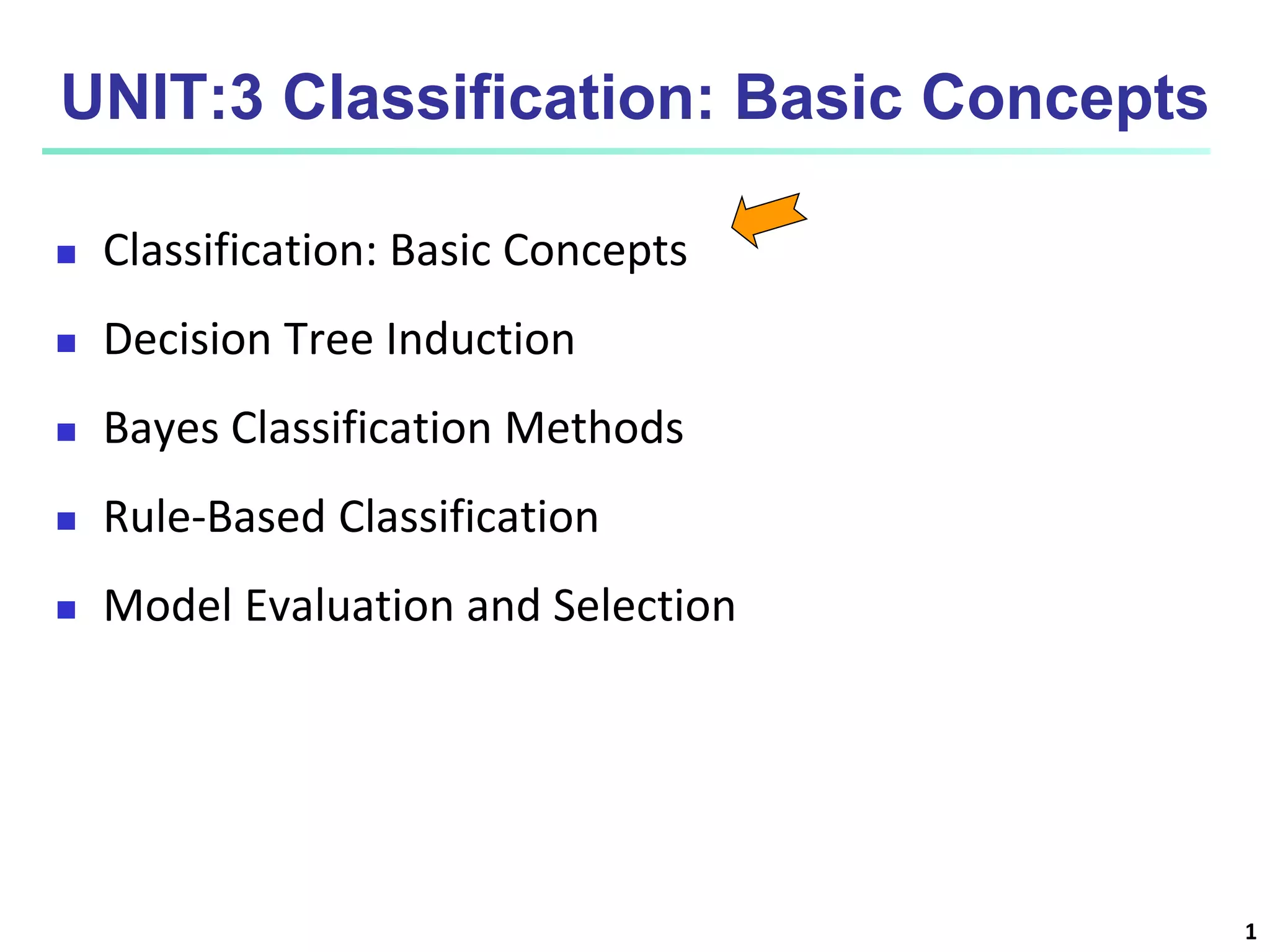
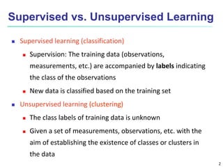
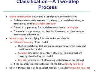
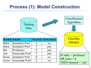
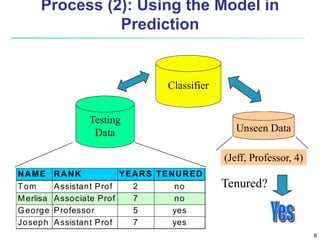
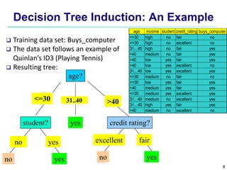
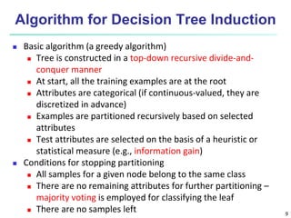
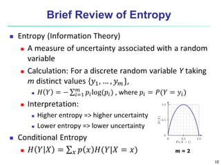
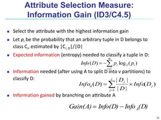
This document provides an overview of classification techniques in machine learning. It discusses: - The process of classification involves model construction using a training set and then applying the model to classify new data. - Supervised learning aims to predict categorical labels while unsupervised learning groups data without labels. - Popular classification algorithms covered include decision trees, Bayesian classification, and rule-based methods. Attribute selection measures, model evaluation, overfitting, and tree pruning are also discussed.

1. 1
UNIT:3 Classification: Basic Concepts
 Classification: Basic Concepts
 Decision Tree Induction
 Bayes Classification Methods
 Rule-Based Classification
 Model Evaluation and Selection

2. 2
Supervised vs. Unsupervised Learning
 Supervised learning (classification)
 Supervision: The training data (observations,
measurements, etc.) are accompanied by labels indicating
the class of the observations
 New data is classified based on the training set
 Unsupervised learning (clustering)
 The class labels of training data is unknown
 Given a set of measurements, observations, etc. with the
aim of establishing the existence of classes or clusters in
the data

3. 3
 Classification
 predicts categorical class labels (discrete or nominal)
 classifies data (constructs a model) based on the training
set and the values (class labels) in a classifying attribute
and uses it in classifying new data
 Numeric Prediction
 models continuous-valued functions, i.e., predicts
unknown or missing values
 Typical applications
 Credit/loan approval:
 Medical diagnosis: if a tumor is cancerous or benign
 Fraud detection: if a transaction is fraudulent
 Web page categorization: which category it is
Prediction Problems: Classification vs.
Numeric Prediction

4. 4
Classification—A Two-Step
Process
 Model construction: describing a set of predetermined classes
 Each tuple/sample is assumed to belong to a predefined class, as
determined by the class label attribute
 The set of tuples used for model construction is training set
 The model is represented as classification rules, decision trees, or
mathematical formulae
 Model usage: for classifying future or unknown objects
 Estimate accuracy of the model
 The known label of test sample is compared with the classified
result from the model
 Accuracy rate is the percentage of test set samples that are
correctly classified by the model
 Test set is independent of training set (otherwise overfitting)
 If the accuracy is acceptable, use the model to classify new data
 Note: If the test set is used to select models, it is called validation (test) set

5. 5
Process (1): Model Construction
Training
Data
NAME RANK YEARS TENURED
Mike Assistant Prof 3 no
Mary Assistant Prof 7 yes
Bill Professor 2 yes
Jim Associate Prof 7 yes
Dave Assistant Prof 6 no
Anne Associate Prof 3 no
Classification
Algorithms
IF rank = ‘professor’
OR years > 6
THEN tenured = ‘yes’
Classifier
(Model)

6. 6
Process (2): Using the Model in
Prediction
Classifier
Testing
Data
NAME RANK YEARS TENURED
Tom Assistant Prof 2 no
Merlisa Associate Prof 7 no
George Professor 5 yes
Joseph Assistant Prof 7 yes
Unseen Data
(Jeff, Professor, 4)
Tenured?

7. 7
Chapter 8. Classification: Basic
Concepts
 Classification: Basic Concepts
 Decision Tree Induction
 Bayes Classification Methods
 Rule-Based Classification
 Model Evaluation and Selection
 Techniques to Improve Classification Accuracy:
Ensemble Methods
 Summary

8. 8
Decision Tree Induction: An Example
age?
overcast
student? credit rating?
<=30 >40
no yes yes
yes
31..40
fairexcellentyesno
age income student credit_rating buys_computer
<=30 high no fair no
<=30 high no excellent no
31…40 high no fair yes
>40 medium no fair yes
>40 low yes fair yes
>40 low yes excellent no
31…40 low yes excellent yes
<=30 medium no fair no
<=30 low yes fair yes
>40 medium yes fair yes
<=30 medium yes excellent yes
31…40 medium no excellent yes
31…40 high yes fair yes
>40 medium no excellent no
 Training data set: Buys_computer
 The data set follows an example of
Quinlan’s ID3 (Playing Tennis)
 Resulting tree:

9. 9
Algorithm for Decision Tree Induction
 Basic algorithm (a greedy algorithm)
 Tree is constructed in a top-down recursive divide-and-
conquer manner
 At start, all the training examples are at the root
 Attributes are categorical (if continuous-valued, they are
discretized in advance)
 Examples are partitioned recursively based on selected
attributes
 Test attributes are selected on the basis of a heuristic or
statistical measure (e.g., information gain)
 Conditions for stopping partitioning
 All samples for a given node belong to the same class
 There are no remaining attributes for further partitioning –
majority voting is employed for classifying the leaf
 There are no samples left

10. Brief Review of Entropy

10
m = 2

11. 11
Attribute Selection Measure:
Information Gain (ID3/C4.5)
 Select the attribute with the highest information gain
 Let pi be the probability that an arbitrary tuple in D belongs to
class Ci, estimated by |Ci, D|/|D|
 Expected information (entropy) needed to classify a tuple in D:
 Information needed (after using A to split D into v partitions) to
classify D:
 Information gained by branching on attribute A
)(log)( 2
1
i
m
i
i ppDInfo 

)(
||
||
)(
1
j
v
j
j
A DInfo
D
D
DInfo  
(D)InfoInfo(D)Gain(A) A

12. 12
Attribute Selection: Information Gain
 Class P: buys_computer = “yes”
 Class N: buys_computer = “no”
means “age <=30” has 5 out of
14 samples, with 2 yes’es and 3
no’s. Hence
Similarly,
age pi ni I(pi, ni)
<=30 2 3 0.971
31…40 4 0 0
>40 3 2 0.971
694.0)2,3(
14
5
)0,4(
14
4
)3,2(
14
5
)(


I
IIDInfoage
048.0)_(
151.0)(
029.0)(



ratingcreditGain
studentGain
incomeGain
246.0)()()(  DInfoDInfoageGain age
age income student credit_rating buys_computer
<=30 high no fair no
<=30 high no excellent no
31…40 high no fair yes
>40 medium no fair yes
>40 low yes fair yes
>40 low yes excellent no
31…40 low yes excellent yes
<=30 medium no fair no
<=30 low yes fair yes
>40 medium yes fair yes
<=30 medium yes excellent yes
31…40 medium no excellent yes
31…40 high yes fair yes
>40 medium no excellent no
)3,2(
14
5
I
940.0)
14
5
(log
14
5
)
14
9
(log
14
9
)5,9()( 22  IDInfo

13. 13
Computing Information-Gain for
Continuous-Valued Attributes
 Let attribute A be a continuous-valued attribute
 Must determine the best split point for A
 Sort the value A in increasing order
 Typically, the midpoint between each pair of adjacent values
is considered as a possible split point
 (ai+ai+1)/2 is the midpoint between the values of ai and ai+1
 The point with the minimum expected information
requirement for A is selected as the split-point for A
 Split:
 D1 is the set of tuples in D satisfying A ≤ split-point, and D2 is
the set of tuples in D satisfying A > split-point

14. 14
Gain Ratio for Attribute Selection
(C4.5)
 Information gain measure is biased towards attributes with a
large number of values
 C4.5 (a successor of ID3) uses gain ratio to overcome the
problem (normalization to information gain)
 GainRatio(A) = Gain(A)/SplitInfo(A)
 Ex.
 gain_ratio(income) = 0.029/1.557 = 0.019
 The attribute with the maximum gain ratio is selected as the
splitting attribute
)
||
||
(log
||
||
)( 2
1 D
D
D
D
DSplitInfo
j
v
j
j
A  

15. 15
Gini Index (CART, IBM
IntelligentMiner)
 If a data set D contains examples from n classes, gini index,
gini(D) is defined as
where pj is the relative frequency of class j in D
 If a data set D is split on A into two subsets D1 and D2, the gini
index gini(D) is defined as
 Reduction in Impurity:
 The attribute provides the smallest ginisplit(D) (or the largest
reduction in impurity) is chosen to split the node (need to
enumerate all the possible splitting points for each attribute)



n
j
p jDgini
1
21)(
)(
||
||
)(
||
||
)( 2
2
1
1
Dgini
D
D
Dgini
D
D
DginiA

)()()( DginiDginiAgini A


16. 16
Computation of Gini Index
 Ex. D has 9 tuples in buys_computer = “yes” and 5 in “no”
 Suppose the attribute income partitions D into 10 in D1: {low,
medium} and 4 in D2
Gini{low,high} is 0.458; Gini{medium,high} is 0.450. Thus, split on the
{low,medium} (and {high}) since it has the lowest Gini index
 All attributes are assumed continuous-valued
 May need other tools, e.g., clustering, to get the possible split
values
 Can be modified for categorical attributes
459.0
14
5
14
9
1)(
22












Dgini
)(
14
4
)(
14
10
)( 21},{ DGiniDGiniDgini mediumlowincome 













17. 17
Comparing Attribute Selection Measures
 The three measures, in general, return good results but
 Information gain:
 biased towards multivalued attributes
 Gain ratio:
 tends to prefer unbalanced splits in which one partition is
much smaller than the others
 Gini index:
 biased to multivalued attributes
 has difficulty when # of classes is large
 tends to favor tests that result in equal-sized partitions
and purity in both partitions

18. 18
Other Attribute Selection Measures
 CHAID: a popular decision tree algorithm, measure based on χ2 test for
independence
 C-SEP: performs better than info. gain and gini index in certain cases
 G-statistic: has a close approximation to χ2 distribution
 MDL (Minimal Description Length) principle (i.e., the simplest solution is
preferred):
 The best tree as the one that requires the fewest # of bits to both (1)
encode the tree, and (2) encode the exceptions to the tree
 Multivariate splits (partition based on multiple variable combinations)
 CART: finds multivariate splits based on a linear comb. of attrs.
 Which attribute selection measure is the best?
 Most give good results, none is significantly superior than others

19. 19
Overfitting and Tree Pruning
 Overfitting: An induced tree may overfit the training data
 Too many branches, some may reflect anomalies due to
noise or outliers
 Poor accuracy for unseen samples
 Two approaches to avoid overfitting
 Prepruning: Halt tree construction early ̵ do not split a node
if this would result in the goodness measure falling below a
threshold
 Difficult to choose an appropriate threshold
 Postpruning: Remove branches from a “fully grown” tree—
get a sequence of progressively pruned trees
 Use a set of data different from the training data to
decide which is the “best pruned tree”

20. 20
Enhancements to Basic Decision Tree
Induction
 Allow for continuous-valued attributes
 Dynamically define new discrete-valued attributes that
partition the continuous attribute value into a discrete set of
intervals
 Handle missing attribute values
 Assign the most common value of the attribute
 Assign probability to each of the possible values
 Attribute construction
 Create new attributes based on existing ones that are
sparsely represented
 This reduces fragmentation, repetition, and replication

21. 21
Classification in Large Databases
 Classification—a classical problem extensively studied by
statisticians and machine learning researchers
 Scalability: Classifying data sets with millions of examples and
hundreds of attributes with reasonable speed
 Why is decision tree induction popular?
 relatively faster learning speed (than other classification
methods)
 convertible to simple and easy to understand classification
rules
 can use SQL queries for accessing databases
 comparable classification accuracy with other methods
 RainForest (VLDB’98 — Gehrke, Ramakrishnan & Ganti)
 Builds an AVC-list (attribute, value, class label)

22. 22
Chapter 8. Classification: Basic
Concepts
 Classification: Basic Concepts
 Decision Tree Induction
 Bayes Classification Methods
 Rule-Based Classification
 Model Evaluation and Selection
 Techniques to Improve Classification Accuracy:
Ensemble Methods
 Summary

23. 23
Bayesian Classification: Why?
 A statistical classifier: performs probabilistic prediction, i.e.,
predicts class membership probabilities
 Foundation: Based on Bayes’ Theorem.
 Performance: A simple Bayesian classifier, naïve Bayesian
classifier, has comparable performance with decision tree and
selected neural network classifiers
 Incremental: Each training example can incrementally
increase/decrease the probability that a hypothesis is correct —
prior knowledge can be combined with observed data
 Standard: Even when Bayesian methods are computationally
intractable, they can provide a standard of optimal decision
making against which other methods can be measured

24. 24
Bayes’ Theorem: Basics
 Total probability Theorem:
 Bayes’ Theorem:
 Let X be a data sample (“evidence”): class label is unknown
 Let H be a hypothesis that X belongs to class C
 Classification is to determine P(H|X), (i.e., posteriori probability): the
probability that the hypothesis holds given the observed data sample X
 P(H) (prior probability): the initial probability
 E.g., X will buy computer, regardless of age, income, …
 P(X): probability that sample data is observed
 P(X|H) (likelihood): the probability of observing the sample X, given that
the hypothesis holds
 E.g., Given that X will buy computer, the prob. that X is 31..40,
medium income
)()
1
|()(
i
AP
M
i i
ABPBP 


)(/)()|(
)(
)()|()|( XX
X
XX PHPHP
P
HPHPHP 

25. 25
Prediction Based on Bayes’ Theorem
 Given training data X, posteriori probability of a hypothesis H,
P(H|X), follows the Bayes’ theorem
 Informally, this can be viewed as
posteriori = likelihood x prior/evidence
 Predicts X belongs to Ci iff the probability P(Ci|X) is the highest
among all the P(Ck|X) for all the k classes
 Practical difficulty: It requires initial knowledge of many
probabilities, involving significant computational cost
)(/)()|(
)(
)()|()|( XX
X
XX PHPHP
P
HPHPHP 

26. 26
Naïve Bayes Classifier
 A simplified assumption: attributes are conditionally
independent (i.e., no dependence relation between
attributes):
 This greatly reduces the computation cost: Only counts the
class distribution
 If Ak is categorical, P(xk|Ci) is the # of tuples in Ci having value xk
for Ak divided by |Ci, D| (# of tuples of Ci in D)
 If Ak is continous-valued, P(xk|Ci) is usually computed based on
Gaussian distribution with a mean μ and standard deviation σ
and P(xk|Ci) is
)|(...)|()|(
1
)|()|(
21
CixPCixPCixP
n
k
CixPCiP
nk


X
2
2
2
)(
2
1
),,( 






x
exg
),,()|( ii CCkxgCiP X

27. 27
Naïve Bayes Classifier: Training Dataset
Class:
C1:buys_computer = ‘yes’
C2:buys_computer = ‘no’
Data to be classified:
X = (age <=30,
Income = medium,
Student = yes
Credit_rating = Fair)
age income studentcredit_ratingbuys_compu
<=30 high no fair no
<=30 high no excellent no
31…40 high no fair yes
>40 medium no fair yes
>40 low yes fair yes
>40 low yes excellent no
31…40 low yes excellent yes
<=30 medium no fair no
<=30 low yes fair yes
>40 medium yes fair yes
<=30 medium yes excellent yes
31…40 medium no excellent yes
31…40 high yes fair yes
>40 medium no excellent no

28. 28
Naïve Bayes Classifier: An Example
 P(Ci): P(buys_computer = “yes”) = 9/14 = 0.643
P(buys_computer = “no”) = 5/14= 0.357
 Compute P(X|Ci) for each class
P(age = “<=30” | buys_computer = “yes”) = 2/9 = 0.222
P(age = “<= 30” | buys_computer = “no”) = 3/5 = 0.6
P(income = “medium” | buys_computer = “yes”) = 4/9 = 0.444
P(income = “medium” | buys_computer = “no”) = 2/5 = 0.4
P(student = “yes” | buys_computer = “yes) = 6/9 = 0.667
P(student = “yes” | buys_computer = “no”) = 1/5 = 0.2
P(credit_rating = “fair” | buys_computer = “yes”) = 6/9 = 0.667
P(credit_rating = “fair” | buys_computer = “no”) = 2/5 = 0.4
 X = (age <= 30 , income = medium, student = yes, credit_rating = fair)
P(X|Ci) : P(X|buys_computer = “yes”) = 0.222 x 0.444 x 0.667 x 0.667 = 0.044
P(X|buys_computer = “no”) = 0.6 x 0.4 x 0.2 x 0.4 = 0.019
P(X|Ci)*P(Ci) : P(X|buys_computer = “yes”) * P(buys_computer = “yes”) = 0.028
P(X|buys_computer = “no”) * P(buys_computer = “no”) = 0.007
Therefore, X belongs to class (“buys_computer = yes”)
age income studentcredit_ratingbuys_comp
<=30 high no fair no
<=30 high no excellent no
31…40 high no fair yes
>40 medium no fair yes
>40 low yes fair yes
>40 low yes excellent no
31…40 low yes excellent yes
<=30 medium no fair no
<=30 low yes fair yes
>40 medium yes fair yes
<=30 medium yes excellent yes
31…40 medium no excellent yes
31…40 high yes fair yes
>40 medium no excellent no

29. 29
Naïve Bayes Classifier: Comments
 Advantages
 Easy to implement
 Good results obtained in most of the cases
 Disadvantages
 Assumption: class conditional independence, therefore loss
of accuracy
 Practically, dependencies exist among variables
 E.g., hospitals: patients: Profile: age, family history, etc.
Symptoms: fever, cough etc., Disease: lung cancer,
diabetes, etc.
 Dependencies among these cannot be modeled by Naïve
Bayes Classifier
 How to deal with these dependencies? Bayesian Belief Networks
(Chapter 9)

30. 30
Chapter 8. Classification: Basic
Concepts
 Classification: Basic Concepts
 Decision Tree Induction
 Bayes Classification Methods
 Rule-Based Classification
 Model Evaluation and Selection
 Techniques to Improve Classification Accuracy:
Ensemble Methods
 Summary

31. 31
Using IF-THEN Rules for Classification
 Represent the knowledge in the form of IF-THEN rules
R: IF age = youth AND student = yes THEN buys_computer = yes
 Rule antecedent/precondition vs. rule consequent
 Assessment of a rule: coverage and accuracy
 ncovers = # of tuples covered by R
 ncorrect = # of tuples correctly classified by R
coverage(R) = ncovers /|D| /* D: training data set */
accuracy(R) = ncorrect / ncovers
 If more than one rule are triggered, need conflict resolution
 Size ordering: assign the highest priority to the triggering rules that has
the “toughest” requirement (i.e., with the most attribute tests)
 Class-based ordering: decreasing order of prevalence or misclassification
cost per class
 Rule-based ordering (decision list): rules are organized into one long
priority list, according to some measure of rule quality or by experts

32. 32
age?
student? credit rating?
<=30 >40
no yes yes
yes
31..40
fairexcellentyesno
 Example: Rule extraction from our buys_computer decision-tree
IF age = young AND student = no THEN buys_computer = no
IF age = young AND student = yes THEN buys_computer = yes
IF age = mid-age THEN buys_computer = yes
IF age = old AND credit_rating = excellent THEN buys_computer = no
IF age = old AND credit_rating = fair THEN buys_computer = yes
Rule Extraction from a Decision Tree
 Rules are easier to understand than large
trees
 One rule is created for each path from the
root to a leaf
 Each attribute-value pair along a path forms a
conjunction: the leaf holds the class
prediction
 Rules are mutually exclusive and exhaustive

33. 33
Rule Induction: Sequential Covering
Method
 Sequential covering algorithm: Extracts rules directly from training
data
 Typical sequential covering algorithms: FOIL, AQ, CN2, RIPPER
 Rules are learned sequentially, each for a given class Ci will cover
many tuples of Ci but none (or few) of the tuples of other classes
 Steps:
 Rules are learned one at a time
 Each time a rule is learned, the tuples covered by the rules are
removed
 Repeat the process on the remaining tuples until termination
condition, e.g., when no more training examples or when the
quality of a rule returned is below a user-specified threshold
 Comp. w. decision-tree induction: learning a set of rules
simultaneously

34. Issues Affecting Model Selection
 Accuracy
 classifier accuracy: predicting class label
 Speed
 time to construct the model (training time)
 time to use the model (classification/prediction time)
 Robustness: handling noise and missing values
 Scalability: efficiency in disk-resident databases
 Interpretability
 understanding and insight provided by the model
 Other measures, e.g., goodness of rules, such as decision tree
size or compactness of classification rules
34

35. 35
Issues: Evaluating Classification Methods
 Accuracy
 classifier accuracy: predicting class label
 predictor accuracy: guessing value of predicted attributes
 Speed
 time to construct the model (training time)
 time to use the model (classification/prediction time)
 Robustness: handling noise and missing values
 Scalability: efficiency in disk-resident databases
 Interpretability
 understanding and insight provided by the model
 Other measures, e.g., goodness of rules, such as decision tree
size or compactness of classification rules