The document discusses decision tree induction algorithms. It begins with an introduction to decision trees, describing their structure and how they are used for classification. It then covers the basic algorithm for constructing decision trees, including the ID3, C4.5, and CART algorithms. Next, it discusses different attribute selection measures that can be used to determine the best attribute to split on at each node, including information gain, gain ratio, and the Gini index. It provides details on how information gain is calculated.

1. 3/1/2012
Outline
 Introduction
 Basic Algorithm for Decision Tree Induction
 Attribute Selection Measures
– Information Gain
– Gain Ratio
– Gini Index
 Tree Pruning
 Scalable Decision Tree Induction Methods
2
1. Introduction
Decision Tree Induction
The Decision Tree is one of the most powerful and popular classification and
prediction algorithms in current use in data mining and machine learning. The
attractiveness of decision trees is due to the fact that, in contrast to neural
networks, decision trees represent rules. Rules can readily be expressed so that
humans can understand them or even directly used in a database access language
like SQL so that records falling into a particular category may be retrieved.
• A decision tree is a flowchart classifier like tree structure, where
– each internal node (non-leaf node, decision node) denotes a test on an attribute
– each branch represents an outcome of the test
– each leaf node (or terminal node) indicates the value of the target attribute
(class) of examples.
3
– The topmost node in a tree is the root node
1

2. 3/1/2012
A decision tree consists of nodes and arcs which connect nodes. To make a
decision, one starts at the root node, and asks questions to determine
which arc to follow, until one reaches a leaf node and the decision is made.
How are decision trees used for classification?
– Given an instance, X, for which the associated class label is unknown
– The attribute values of the instance are tested against the decision tree
– A path is traced from the root to a leaf node, which holds the class prediction
for that instance.
Applications
Decision tree algorithms have been used for classification in many
application areas, such as:
– Medicine
– Manufacturing and production
– Financial analysis
– Astronomy
– Molecular biology. 4
• Advantages of decision tree
– The construction of decision tree classifiers does not parameter
setting.
– Decision trees can handle high dimensional data.
– Easy to interpret for small-sized trees
– The learning and classification steps of decision tree induction
are simple and fast.
– Accuracy is comparable to other classification techniques for
many simple data sets
– Convertible to simple and easy to understand classification rules
5
2

3. 3/1/2012
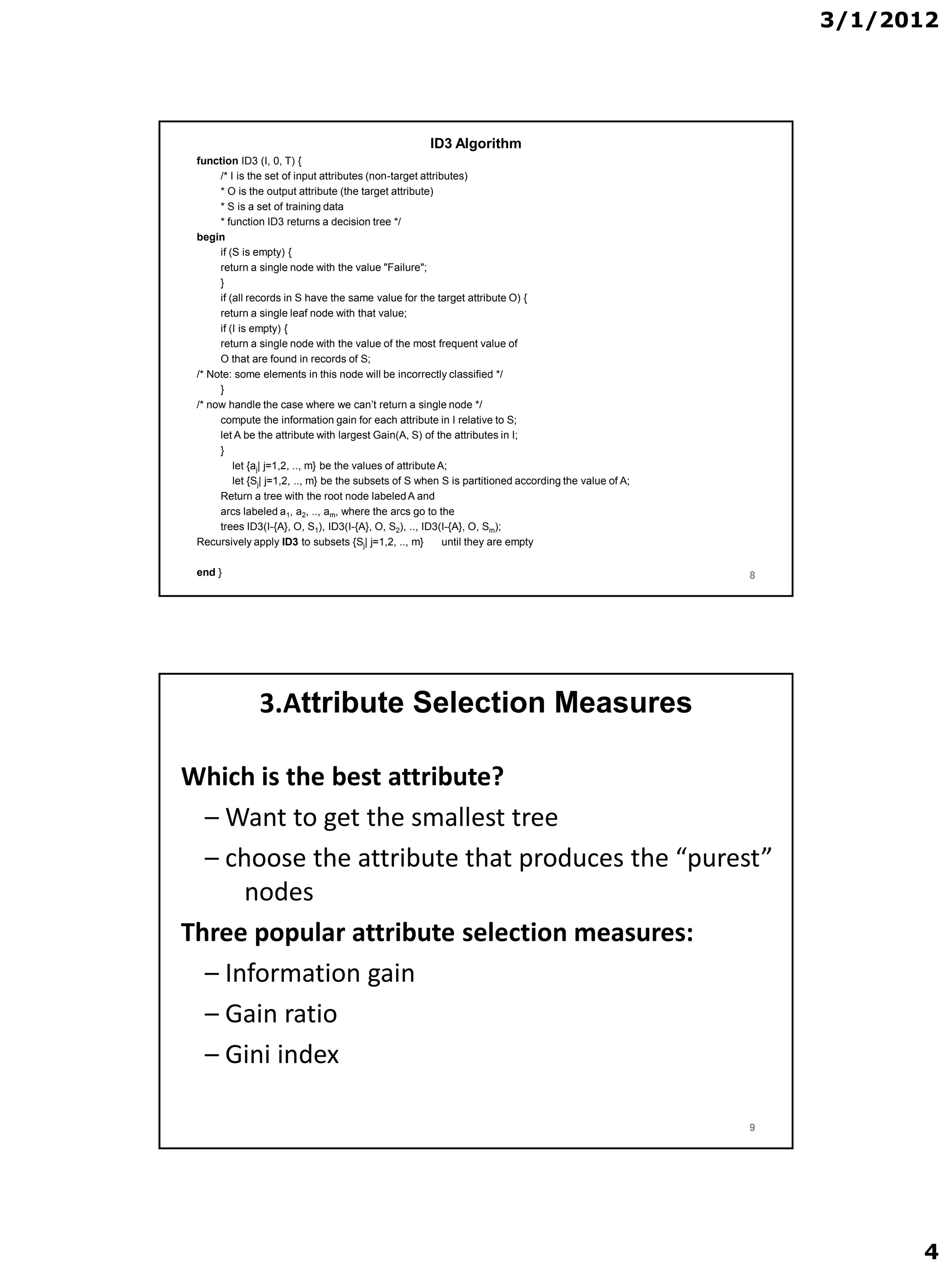
2. Basic Algorithm
Decision Tree Algorithms
• ID3 algorithm
• C4.5 algorithm
- A successor of ID3
– Became a benchmark to which newer supervised learning
algorithms are often compared.
– Commercial successor: C5.0
• CART (Classification and Regression Trees) algorithm
– The generation of binary decision trees
– Developed by a group of statisticians
6
Basic Algorithm
• Basic algorithm ,[ID3, C4.5, and CART], (a greedy algorithm)
– Tree is constructed in a top-down recursive divide-and-
conquer manner
– At start, all the training examples are at the root
– Attributes are categorical (if continuous-valued, they are
discretized in advance)
– Examples are partitioned recursively into smaller subsets as
the tree is being built based on selected attributes
– Test attributes are selected on the basis of a statistical
measure (e.g., information gain)
7
3

4. 3/1/2012
ID3 Algorithm
function ID3 (I, 0, T) {
/* I is the set of input attributes (non-target attributes)
* O is the output attribute (the target attribute)
* S is a set of training data
* function ID3 returns a decision tree */
begin
if (S is empty) {
return a single node with the value "Failure";
}
if (all records in S have the same value for the target attribute O) {
return a single leaf node with that value;
if (I is empty) {
return a single node with the value of the most frequent value of
O that are found in records of S;
/* Note: some elements in this node will be incorrectly classified */
}
/* now handle the case where we can’t return a single node */
compute the information gain for each attribute in I relative to S;
let A be the attribute with largest Gain(A, S) of the attributes in I;
}
let {aj| j=1,2, .., m} be the values of attribute A;
let {Sj| j=1,2, .., m} be the subsets of S when S is partitioned according the value of A;
Return a tree with the root node labeled A and
arcs labeled a1, a2, .., am, where the arcs go to the
trees ID3(I-{A}, O, S1), ID3(I-{A}, O, S2), .., ID3(I-{A}, O, Sm);
Recursively apply ID3 to subsets {Sj| j=1,2, .., m} until they are empty
end } 8
3.Attribute Selection Measures
Which is the best attribute?
– Want to get the smallest tree
– choose the attribute that produces the “purest”
nodes
Three popular attribute selection measures:
– Information gain
– Gain ratio
– Gini index
9
4

5. 3/1/2012
Information gain
• The estimation criterion in the decision tree algorithm is the
selection of an attribute to test at each decision node in the
tree.
• The goal is to select the attribute that is most useful for
classifying examples. A good quantitative measure of the
worth of an attribute is a statistical property called information
gain that measures how well a given attribute separates the
training examples according to their target classification.
• This measure is used to select among the candidate
attributes at each step while growing the tree. 10
Entropy - a measure of homogeneity of the set of examples
• In order to define information gain precisely, we need to
define a measure commonly used in information theory,
called entropy (Expected information, info(),).
• Given a set S, containing only positive and negative
examples of some target concept (a 2 class problem), the
entropy of set S relative to this simple, binary classification
is defined as:
Info(S) =
• where pi is the proportion of S belonging to class i. Note the
logarithm is still base 2 because entropy is a measure of the
expected encoding length measured in bits.
• In all calculations involving entropy we define 0log0 to be 0.
11
5

6. 3/1/2012
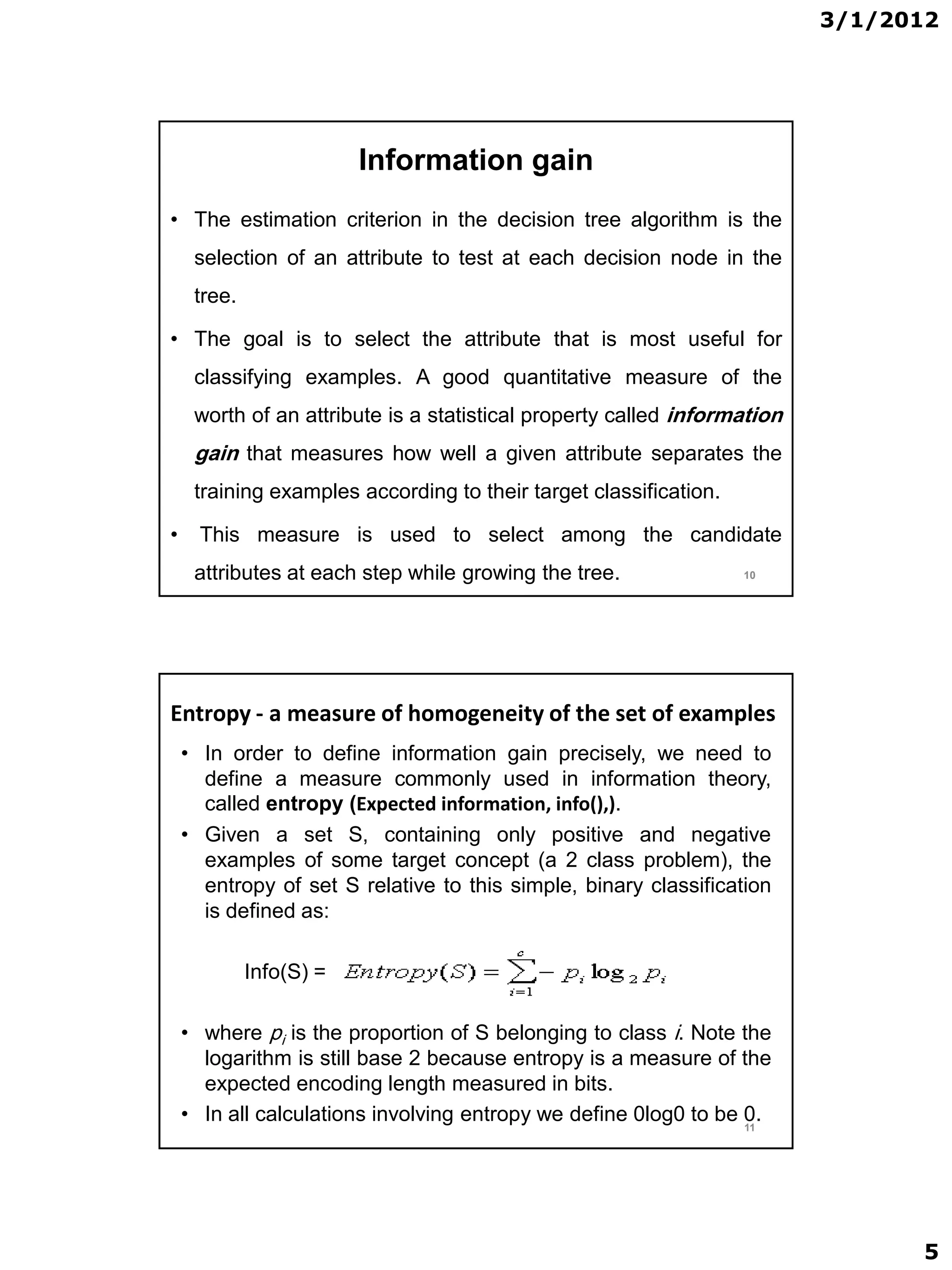
• For example, suppose S is a collection of 25 examples, including 15
positive and 10 negative examples [15+, 10-]. Then the entropy of
S relative to this classification is :
Entropy(S) = - (15/25) log2 (15/25) - (10/25) log2 (10/25) = 0.970
• Notice that the entropy is 0 if all members of S belong to the same
class. For example,
Entropy(S) = -1 log2(1) - 0 log20 = -1 0 - 0 log20 = 0.
• Note the entropy is 1 (at its maximum!) when the collection
contains an equal number of positive and negative examples.
• If the collection contains unequal numbers of positive and
negative examples, the entropy is between 0 and 1. Figure 1
shows the form of the entropy function relative to a binary
classification, as p+ varies between 0 and 1. 12
Figure 1: The entropy function relative to a binary classification, as the proportion of positive
examples pp varies between 0 and 1.
Entropy of S = Info(S)
-The average amount of information needed to identify the class label of an
instance in D.
- A measure of the impurity in a collection of training examples
- The smaller information required, the greater the purity of the partitions.
13
6

7. 3/1/2012
• Information gain measures the expected reduction in entropy caused by
partitioning the examples according to this attribute.
• The information gain, Gain (S, A) of an attribute A, relative to a collection of
examples S, is defined as
= info (S) – infoA (s)
= information needed before splitting – information needed after splitting
• where Values(A) is the set of all possible values for attribute A, and Sv is
the subset of S for which attribute A has value v (i.e., Sv = {s  S | A(s) = v
}). Note the first term in the equation for Gain is just the entropy of the
original collection S and the second term is infoA (S), the expected value of
the entropy after S is partitioned using attribute A
14
An example: Weather Data
The aim of this exercise is to learn how ID3 works. You will do this by building a
decision tree by hand for a small dataset. At the end of this exercise you should
understand how ID3 constructs a decision tree using the concept of Information
Gain. You will be able to use the decision tree you create to make a decision
about new data.
15
7

8. 3/1/2012
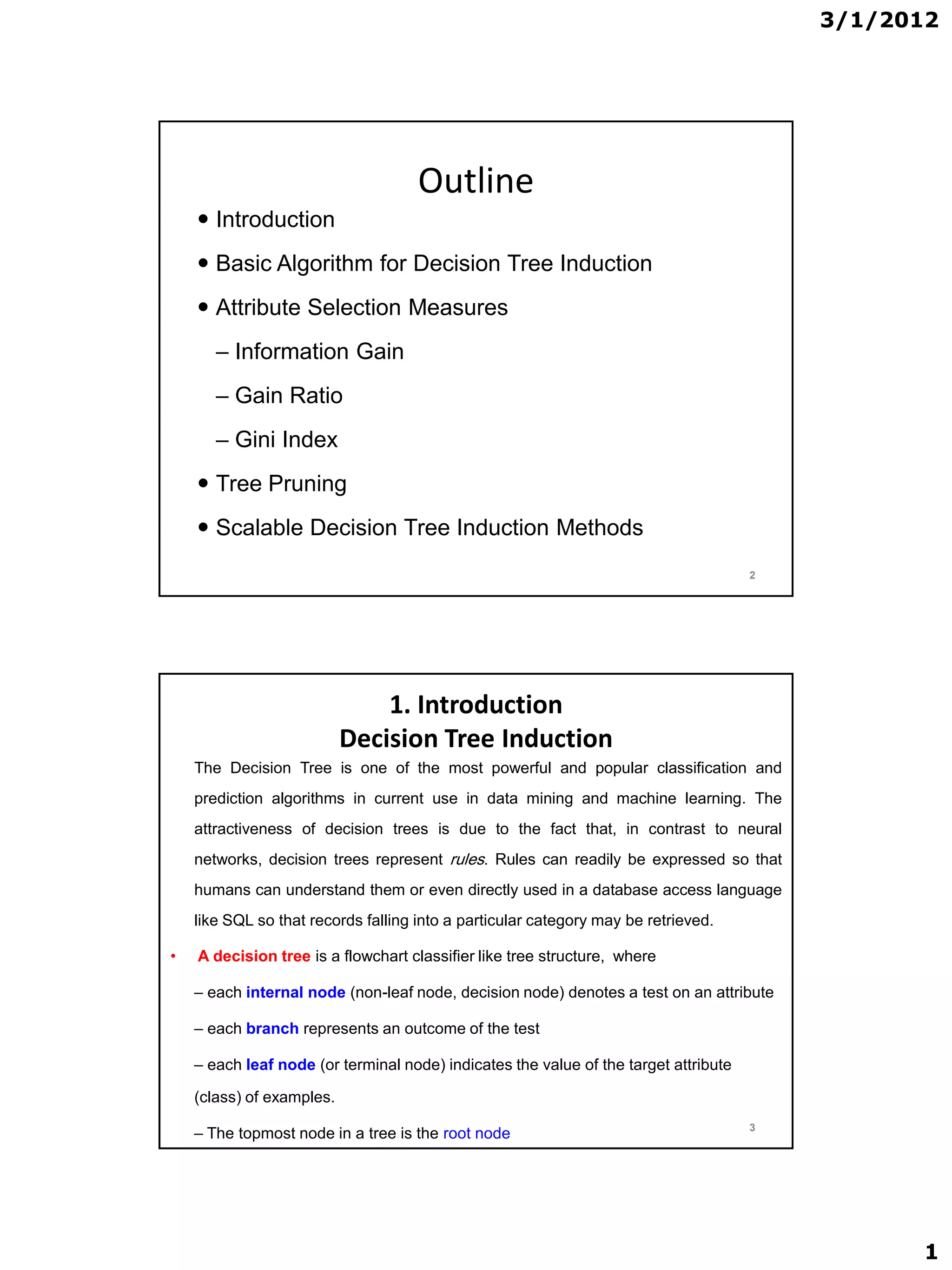
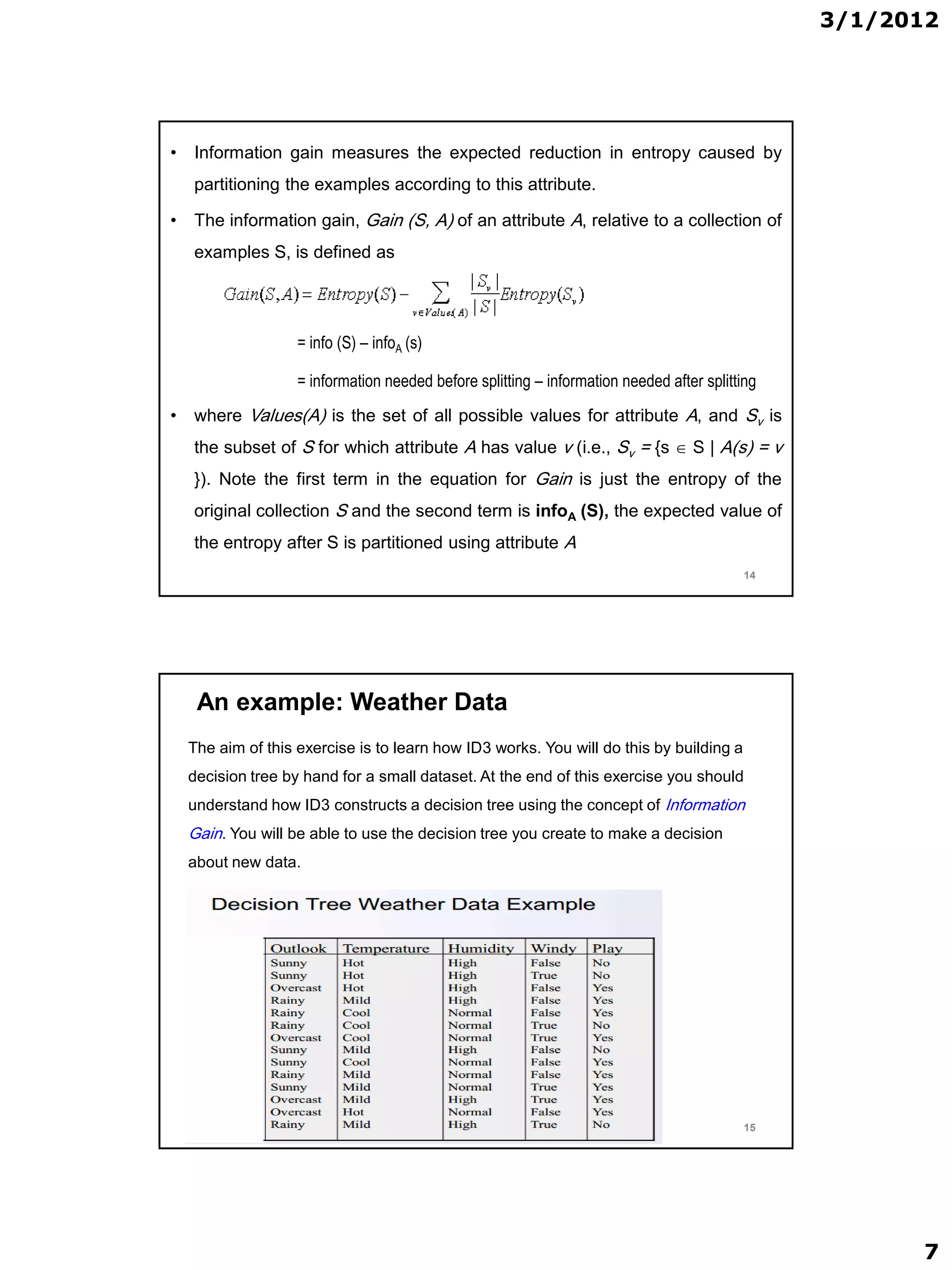
• In this dataset, there are five categorical attributes outlook, temperature,
humidity, windy, and play.
• We are interested in building a system which will enable us to decide
whether or not to play the game on the basis of the weather conditions, i.e.
we wish to predict the value of play using outlook, temperature, humidity,
and windy.
• We can think of the attribute we wish to predict, i.e. play, as the output
attribute, and the other attributes as input attributes.
• In this problem we have 14 examples in which:
9 examples with play= yes and 5 examples with play = no
So, S={9,5}, and
Entropy(S) = info (S) = info([9,5] ) = Entropy(9/14, 5/14)
= -9/14 log2 9/14 – 5/14 log2 5/14 = 0.940
16
consider splitting on Outlook attribute
Outlook = Sunny
info([2; 3]) = entropy(2/5 ; 3/5 ) = -2/5 log2 2/5
- 3/5 log2 3/5 = 0.971 bits
Outlook = Overcast
info([4; 0]) = entropy(4/4,0/4) = -1 log2 1 - 0 log2 0 = 0 bits
Outlook = Rainy
info([3; 2]) = entropy(3/5,2/5)= - 3/5 log2 3/5 – 2/5 log2 2/5 =0.971 bits
So, the expected information needed to classify objects in all sub trees of the
Outlook attribute is :
info outlook (S) = info([2; 3]; [4; 0]; [3; 2]) = 5/14 * 0.971 + 4/14 * 0 + 5/14 * 0.971
= 0.693 bits
information gain = info before split - info after split
gain(Outlook) = info([9; 5]) - info([2; 3]; [4; 0]; [3; 2])
= 0.940 - 0.693 = 0.247 bits
17
8

9. 3/1/2012
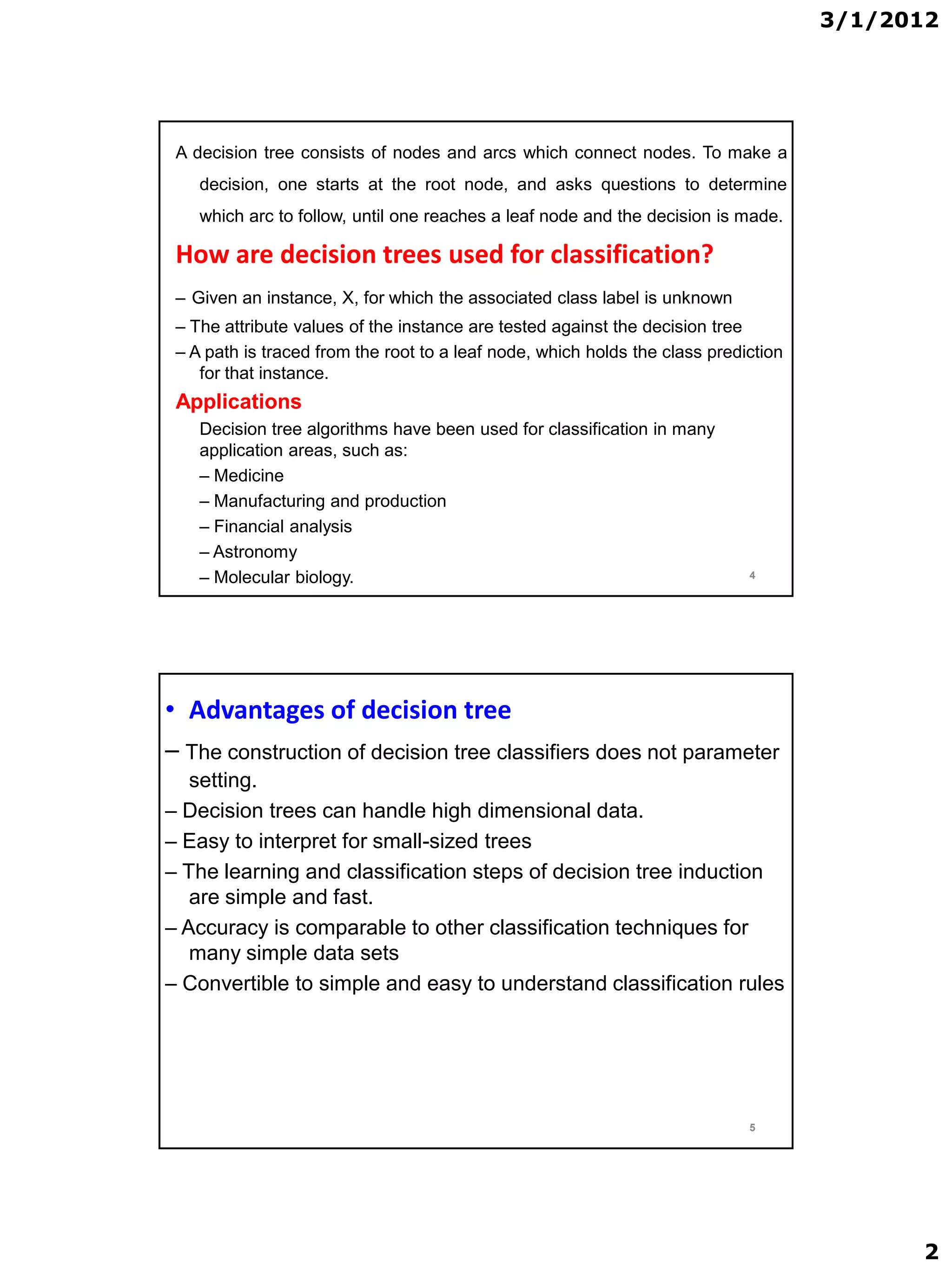
consider splitting on Temperature attribute
temperature = Hot
info([2; 2]) = entropy(2/4 ; 2/4 ) = -2/4 log2 2/4 - 2/4 log2 2/4 =
= 1 bits
temperature = mild
info([4; 2]) = entropy(4/6,2/6) = -4/6 log2 4/6 - 2/6 log2 2/6 =
= 0.918 bits
temperature = cool
info([3; 1]) = entropy(3/4,1/4)= - 3/4 log2 3/4 – 1/4 log2 1/4 =0.881 bits
So, the expected information needed to classify objects in all sub trees of the
temperature attribute is:
info([2; 2]; [4; 2]; [3; 1]) = 4/14 * 1 + 6/14 * 0.981 + 4/14 * 0.881= 0.911 bits
information gain = info before split - info after split
gain(temperature) = 0.940 - 0.911 = 0.029 bits
18
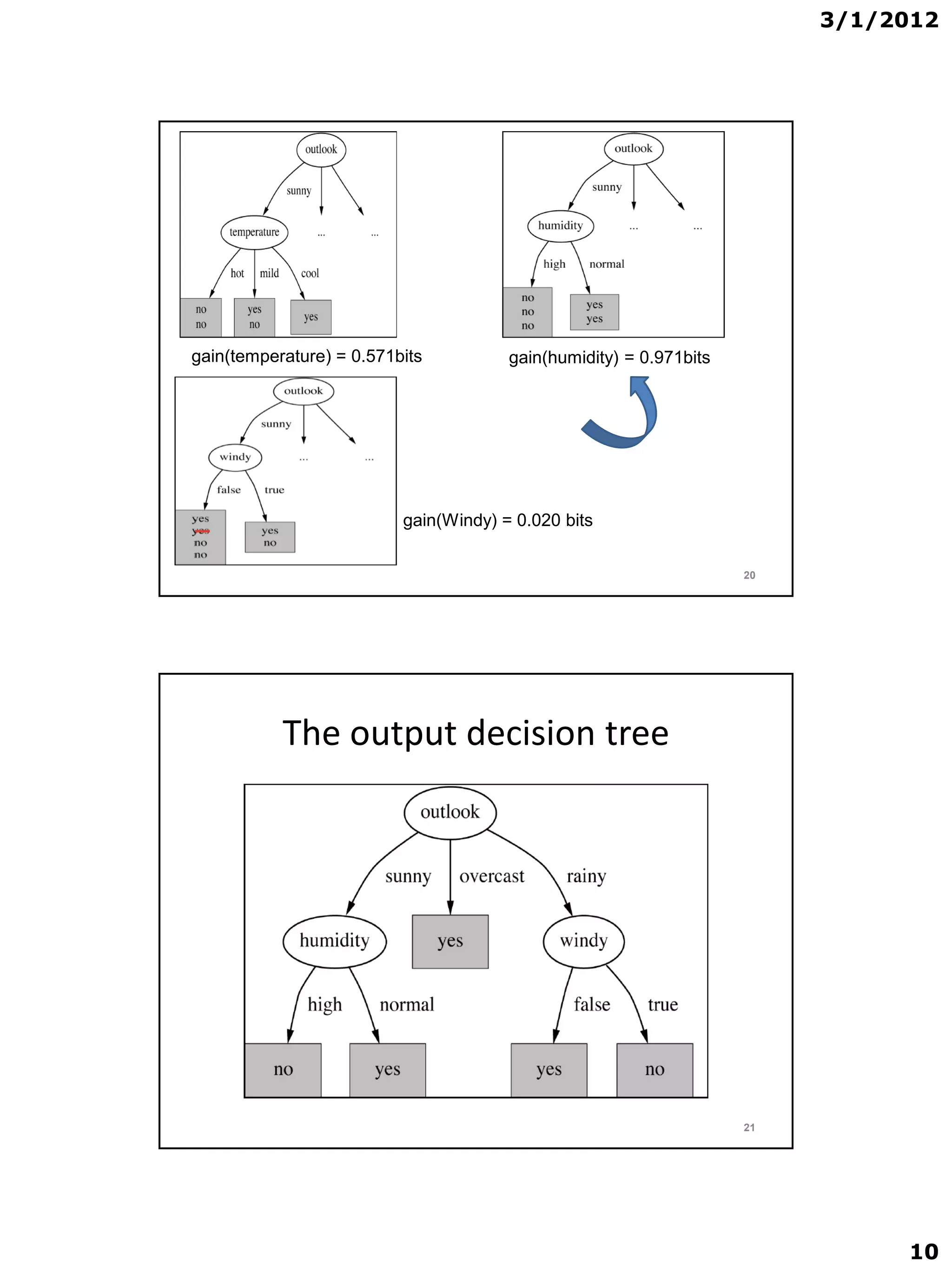
• Complete in the same way we get:
gain(Outlook ) = 0.247 bits
gain(Temperature ) = 0.029 bits
gain(Humidity ) = 0.152 bits
gain(Windy ) = 0.048 bit
• And the selected attribute will be the one with
largest information gain = outlook
• Then Continuing to split …….
19
9

10. 3/1/2012
gain(temperature) = 0.571bits gain(humidity) = 0.971bits
gain(Windy) = 0.020 bits
20
The output decision tree
21
10

11. 3/1/2012
ID3 versus C4.5
• ID3 uses information gain
• C4.5 can use either information gain or gain ratio
• C4.5 can deal with
-numeric/continuous attributes
-missing values
-noisy data
• Alternate method: classification and regression
trees(CART)
22
Decision trees advantages
• Requires little data preparation
• Are able to handle both categorical and numerical data
• Are simple to understand and interpret
• Generate models that can be statistically validated
• The construction of decision tree classifiers does not
parameter setting.
• Decision trees can handle high dimensional data
• perform well with large data in a short time
• The learning and classification steps of decision tree
induction are simple and fast.
• Accuracy is comparable to other classification techniques
for many simple data sets
• Convertible to simple and easy to understand classification
23
rules
11