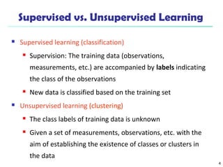
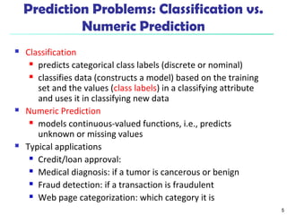
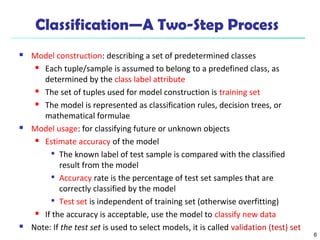
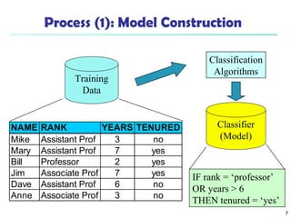
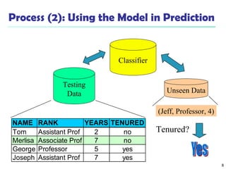
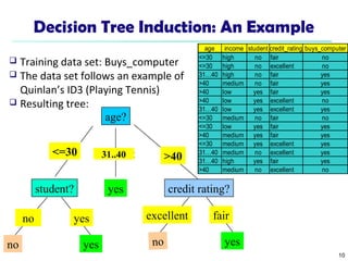
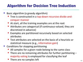
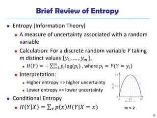
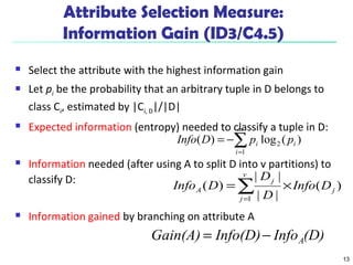
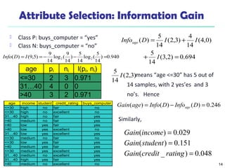
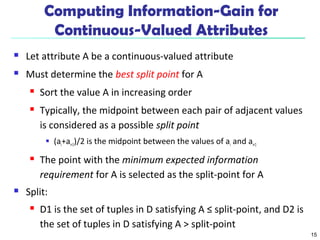
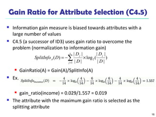
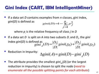
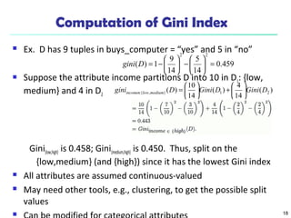
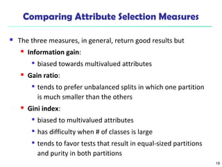
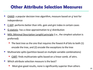
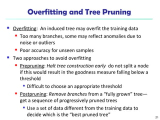
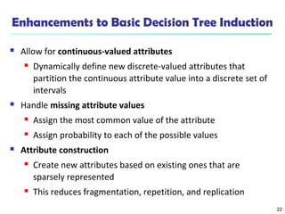
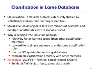
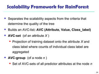
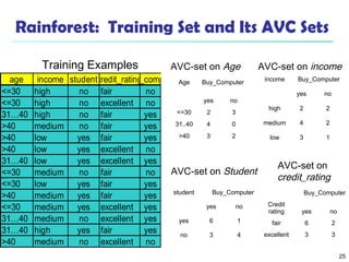
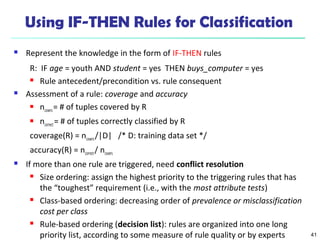
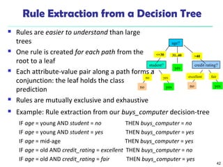
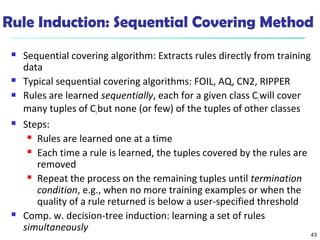
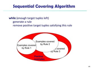
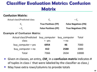
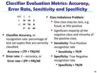
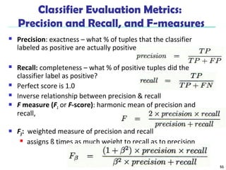
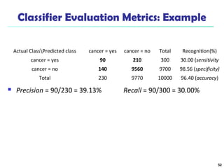
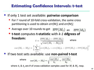
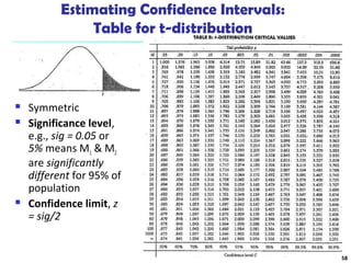
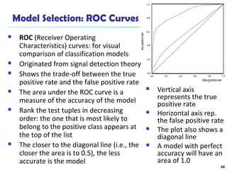
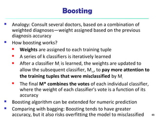
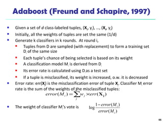
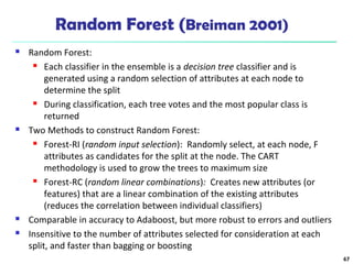
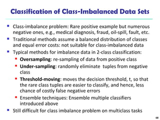
The document summarizes key concepts in classification and decision tree induction. It discusses supervised vs unsupervised learning, the two-step classification process of model construction and usage, and decision tree induction basics including attribute selection measures like information gain, gain ratio, and Gini index. It also covers overfitting and techniques like prepruning and postpruning decision trees.

1. 1
Data Mining:
Concepts and Techniques
(3rd
ed.)
— Chapter 8 —
Jiawei Han, Micheline Kamber, and Jian Pei
University of Illinois at Urbana-Champaign &
Simon Fraser University
©2011 Han, Kamber & Pei. All rights reserved.

3. 3
Chapter 8. Classification: Basic Concepts
 Classification: Basic Concepts
 Decision Tree Induction
 Bayes Classification Methods
 Rule-Based Classification
 Model Evaluation and Selection
 Techniques to Improve Classification Accuracy:
Ensemble Methods
 Summary

4. 4
Supervised vs. Unsupervised Learning
 Supervised learning (classification)
 Supervision: The training data (observations,
measurements, etc.) are accompanied by labels indicating
the class of the observations
 New data is classified based on the training set
 Unsupervised learning (clustering)
 The class labels of training data is unknown
 Given a set of measurements, observations, etc. with the
aim of establishing the existence of classes or clusters in
the data

5. 5
 Classification
 predicts categorical class labels (discrete or nominal)
 classifies data (constructs a model) based on the training
set and the values (class labels) in a classifying attribute
and uses it in classifying new data
 Numeric Prediction
 models continuous-valued functions, i.e., predicts
unknown or missing values
 Typical applications
 Credit/loan approval:
 Medical diagnosis: if a tumor is cancerous or benign
 Fraud detection: if a transaction is fraudulent
 Web page categorization: which category it is
Prediction Problems: Classification vs.
Numeric Prediction

6. 6
Classification—A Two-Step Process
 Model construction: describing a set of predetermined classes
 Each tuple/sample is assumed to belong to a predefined class, as
determined by the class label attribute
 The set of tuples used for model construction is training set
 The model is represented as classification rules, decision trees, or
mathematical formulae
 Model usage: for classifying future or unknown objects
 Estimate accuracy of the model

The known label of test sample is compared with the classified
result from the model

Accuracy rate is the percentage of test set samples that are
correctly classified by the model

Test set is independent of training set (otherwise overfitting)
 If the accuracy is acceptable, use the model to classify new data
 Note: If the test set is used to select models, it is called validation (test) set

7. 7
Process (1): Model Construction
Training
Data
NAME RANK YEARS TENURED
Mike Assistant Prof 3 no
Mary Assistant Prof 7 yes
Bill Professor 2 yes
Jim Associate Prof 7 yes
Dave Assistant Prof 6 no
Anne Associate Prof 3 no
Classification
Algorithms
IF rank = ‘professor’
OR years > 6
THEN tenured = ‘yes’
Classifier
(Model)

8. 8
Process (2): Using the Model in Prediction
Classifier
Testing
Data
NAME RANK YEARS TENURED
Tom Assistant Prof 2 no
Merlisa Associate Prof 7 no
George Professor 5 yes
Joseph Assistant Prof 7 yes
Unseen Data
(Jeff, Professor, 4)
Tenured?

9. 9
Chapter 8. Classification: Basic Concepts
 Classification: Basic Concepts
 Decision Tree Induction
 Bayes Classification Methods
 Rule-Based Classification
 Model Evaluation and Selection
 Techniques to Improve Classification Accuracy:
Ensemble Methods
 Summary

10. 10
Decision Tree Induction: An Example
age?
overcast
student? credit rating?
<=30 >40
no yes yes
yes
31..40
no
fairexcellentyesno
age income student credit_rating buys_computer
<=30 high no fair no
<=30 high no excellent no
31…40 high no fair yes
>40 medium no fair yes
>40 low yes fair yes
>40 low yes excellent no
31…40 low yes excellent yes
<=30 medium no fair no
<=30 low yes fair yes
>40 medium yes fair yes
<=30 medium yes excellent yes
31…40 medium no excellent yes
31…40 high yes fair yes
>40 medium no excellent no
 Training data set: Buys_computer
 The data set follows an example of
Quinlan’s ID3 (Playing Tennis)
 Resulting tree:

11. 11
Algorithm for Decision Tree Induction
 Basic algorithm (a greedy algorithm)
 Tree is constructed in a top-down recursive divide-and-
conquer manner
 At start, all the training examples are at the root
 Attributes are categorical (if continuous-valued, they are
discretized in advance)
 Examples are partitioned recursively based on selected
attributes
 Test attributes are selected on the basis of a heuristic or
statistical measure (e.g., information gain)
 Conditions for stopping partitioning
 All samples for a given node belong to the same class
 There are no remaining attributes for further partitioning –
majority voting is employed for classifying the leaf
 There are no samples left

12. Brief Review of Entropy
12
m = 2

13. 13
Attribute Selection Measure:
Information Gain (ID3/C4.5)
 Select the attribute with the highest information gain
 Let pi be the probability that an arbitrary tuple in D belongs to
class Ci, estimated by |Ci, D|/|D|
 Expected information (entropy) needed to classify a tuple in D:
 Information needed (after using A to split D into v partitions) to
classify D:
 Information gained by branching on attribute A
)(log)( 2
1
i
m
i
i ppDInfo ∑=
−=
)(
||
||
)(
1
j
v
j
j
A DInfo
D
D
DInfo ×= ∑=
(D)InfoInfo(D)Gain(A) A−=

14. 14
Attribute Selection: Information Gain
 Class P: buys_computer = “yes”
 Class N: buys_computer = “no”
means “age <=30” has 5 out of
14 samples, with 2 yes’es and 3
no’s. Hence
Similarly,
age pi ni I(pi, ni)
<=30 2 3 0.971
31…40 4 0 0
>40 3 2 0.971
694.0)2,3(
14
5
)0,4(
14
4
)3,2(
14
5
)(
=+
+=
I
IIDInfoage
048.0)_(
151.0)(
029.0)(
=
=
=
ratingcreditGain
studentGain
incomeGain
246.0)()()( =−= DInfoDInfoageGain age
age income student credit_rating buys_computer
<=30 high no fair no
<=30 high no excellent no
31…40 high no fair yes
>40 medium no fair yes
>40 low yes fair yes
>40 low yes excellent no
31…40 low yes excellent yes
<=30 medium no fair no
<=30 low yes fair yes
>40 medium yes fair yes
<=30 medium yes excellent yes
31…40 medium no excellent yes
31…40 high yes fair yes
>40 medium no excellent no
)3,2(
14
5
I
940.0)
14
5
(log
14
5
)
14
9
(log
14
9
)5,9()( 22 =−−== IDInfo

15. 15
Computing Information-Gain for
Continuous-Valued Attributes
 Let attribute A be a continuous-valued attribute
 Must determine the best split point for A
 Sort the value A in increasing order
 Typically, the midpoint between each pair of adjacent values
is considered as a possible split point
 (ai+ai+1)/2 is the midpoint between the values of ai and ai+1
 The point with the minimum expected information
requirement for A is selected as the split-point for A
 Split:
 D1 is the set of tuples in D satisfying A ≤ split-point, and D2 is
the set of tuples in D satisfying A > split-point

16. 16
Gain Ratio for Attribute Selection (C4.5)
 Information gain measure is biased towards attributes with a
large number of values
 C4.5 (a successor of ID3) uses gain ratio to overcome the
problem (normalization to information gain)
 GainRatio(A) = Gain(A)/SplitInfo(A)
 Ex.
 gain_ratio(income) = 0.029/1.557 = 0.019
 The attribute with the maximum gain ratio is selected as the
splitting attribute
)
||
||
(log
||
||
)( 2
1 D
D
D
D
DSplitInfo
j
v
j
j
A ×−= ∑=

17. 17
Gini Index (CART, IBM IntelligentMiner)
 If a data set D contains examples from n classes, gini index,
gini(D) is defined as
where pj is the relative frequency of class j in D
 If a data set D is split on A into two subsets D1 and D2, the gini
index gini(D) is defined as
 Reduction in Impurity:
 The attribute provides the smallest ginisplit(D) (or the largest
reduction in impurity) is chosen to split the node (need to
enumerate all the possible splitting points for each attribute)
∑
=
−=
n
j
p jDgini
1
21)(
)(
||
||
)(
||
||
)( 2
2
1
1
Dgini
D
D
Dgini
D
D
DginiA
+=
)()()( DginiDginiAgini A
−=∆

18. 18
Computation of Gini Index
 Ex. D has 9 tuples in buys_computer = “yes” and 5 in “no”
 Suppose the attribute income partitions D into 10 in D1: {low,
medium} and 4 in D2
Gini{low,high} is 0.458; Gini{medium,high} is 0.450. Thus, split on the
{low,medium} (and {high}) since it has the lowest Gini index
 All attributes are assumed continuous-valued
 May need other tools, e.g., clustering, to get the possible split
values

459.0
14
5
14
9
1)(
22
=





−





−=Dgini
)(
14
4
)(
14
10
)( 21},{ DGiniDGiniDgini mediumlowincome 





+





=∈

19. 19
Comparing Attribute Selection Measures
 The three measures, in general, return good results but
 Information gain:

biased towards multivalued attributes
 Gain ratio:

tends to prefer unbalanced splits in which one partition
is much smaller than the others
 Gini index:

biased to multivalued attributes

has difficulty when # of classes is large

tends to favor tests that result in equal-sized partitions
and purity in both partitions

20. 20
Other Attribute Selection Measures
 CHAID: a popular decision tree algorithm, measure based on χ2
test for
independence
 C-SEP: performs better than info. gain and gini index in certain cases
 G-statistic: has a close approximation to χ2
distribution
 MDL (Minimal Description Length) principle (i.e., the simplest solution is
preferred):
 The best tree as the one that requires the fewest # of bits to both (1)
encode the tree, and (2) encode the exceptions to the tree
 Multivariate splits (partition based on multiple variable combinations)
 CART: finds multivariate splits based on a linear comb. of attrs.
 Which attribute selection measure is the best?
 Most give good results, none is significantly superior than others

21. 21
Overfitting and Tree Pruning
 Overfitting: An induced tree may overfit the training data
 Too many branches, some may reflect anomalies due to
noise or outliers
 Poor accuracy for unseen samples
 Two approaches to avoid overfitting
 Prepruning: Halt tree construction early do not split a node
if this would result in the goodness measure falling below a
threshold

Difficult to choose an appropriate threshold
 Postpruning: Remove branches from a “fully grown” tree—
get a sequence of progressively pruned trees

Use a set of data different from the training data to
decide which is the “best pruned tree”

22. 22
Enhancements to Basic Decision Tree Induction
 Allow for continuous-valued attributes
 Dynamically define new discrete-valued attributes that
partition the continuous attribute value into a discrete set of
intervals
 Handle missing attribute values
 Assign the most common value of the attribute
 Assign probability to each of the possible values
 Attribute construction
 Create new attributes based on existing ones that are
sparsely represented
 This reduces fragmentation, repetition, and replication

23. 23
Classification in Large Databases
 Classification—a classical problem extensively studied by
statisticians and machine learning researchers
 Scalability: Classifying data sets with millions of examples and
hundreds of attributes with reasonable speed
 Why is decision tree induction popular?
 relatively faster learning speed (than other classification
methods)
 convertible to simple and easy to understand classification
rules
 can use SQL queries for accessing databases
 comparable classification accuracy with other methods
 RainForest (VLDB’98 — Gehrke, Ramakrishnan & Ganti)
 Builds an AVC-list (attribute, value, class label)

24. 24
Scalability Framework for RainForest
 Separates the scalability aspects from the criteria that
determine the quality of the tree
 Builds an AVC-list: AVC (Attribute, Value, Class_label)
 AVC-set (of an attribute X )
 Projection of training dataset onto the attribute X and
class label where counts of individual class label are
aggregated
 AVC-group (of a node n )
 Set of AVC-sets of all predictor attributes at the node n

25. 25
Rainforest: Training Set and Its AVC Sets
student Buy_Computer
yes no
yes 6 1
no 3 4
Age Buy_Computer
yes no
<=30 2 3
31..40 4 0
>40 3 2
Credit
rating
Buy_Computer
yes no
fair 6 2
excellent 3 3
age income studentcredit_ratingbuys_computer
<=30 high no fair no
<=30 high no excellent no
31…40 high no fair yes
>40 medium no fair yes
>40 low yes fair yes
>40 low yes excellent no
31…40 low yes excellent yes
<=30 medium no fair no
<=30 low yes fair yes
>40 medium yes fair yes
<=30 medium yes excellent yes
31…40 medium no excellent yes
31…40 high yes fair yes
>40 medium no excellent no
AVC-set on incomeAVC-set on Age
AVC-set on Student
Training Examples
income Buy_Computer
yes no
high 2 2
medium 4 2
low 3 1
AVC-set on
credit_rating

26. 26
BOAT (Bootstrapped Optimistic
Algorithm for Tree Construction)
 Use a statistical technique called bootstrapping to create
several smaller samples (subsets), each fits in memory
 Each subset is used to create a tree, resulting in several
trees
 These trees are examined and used to construct a new
tree T’
 It turns out that T’ is very close to the tree that would
be generated using the whole data set together
 Adv: requires only two scans of DB, an incremental alg.

27. August 6, 2017 Data Mining: Concepts and Techniques 27
Presentation of Classification Results

28. August 6, 2017 Data Mining: Concepts and Techniques 28
Visualization of a Decision Tree in SGI/MineSet 3.0

29. Data Mining: Concepts and Techniques 29
Interactive Visual Mining by Perception-
Based Classification (PBC)

30. 30
Chapter 8. Classification: Basic Concepts
 Classification: Basic Concepts
 Decision Tree Induction
 Bayes Classification Methods
 Rule-Based Classification
 Model Evaluation and Selection
 Techniques to Improve Classification Accuracy:
Ensemble Methods
 Summary

31. 31
Bayesian Classification: Why?
 A statistical classifier: performs probabilistic prediction, i.e.,
predicts class membership probabilities
 Foundation: Based on Bayes’ Theorem.
 Performance: A simple Bayesian classifier, naïve Bayesian
classifier, has comparable performance with decision tree and
selected neural network classifiers
 Incremental: Each training example can incrementally
increase/decrease the probability that a hypothesis is correct —
prior knowledge can be combined with observed data
 Standard: Even when Bayesian methods are computationally
intractable, they can provide a standard of optimal decision
making against which other methods can be measured

32. 32
Bayes’ Theorem: Basics
 Total probability Theorem:
 Bayes’ Theorem:
 Let X be a data sample (“evidence”): class label is unknown
 Let H be a hypothesis that X belongs to class C
 Classification is to determine P(H|X), (i.e., posteriori probability): the
probability that the hypothesis holds given the observed data sample X
 P(H) (prior probability): the initial probability

E.g., X will buy computer, regardless of age, income, …
 P(X): probability that sample data is observed
 P(X|H) (likelihood): the probability of observing the sample X, given that
the hypothesis holds

E.g., Given that X will buy computer, the prob. that X is 31..40,
medium income
)()
1
|()(
i
AP
M
i i
ABPBP ∑
=
=
)(/)()|(
)(
)()|()|( XX
X
XX PHPHP
P
HPHPHP ×==

33. 33
Prediction Based on Bayes’ Theorem
 Given training data X, posteriori probability of a hypothesis H,
P(H|X), follows the Bayes’ theorem
 Informally, this can be viewed as
posteriori = likelihood x prior/evidence
 Predicts X belongs to Ci iff the probability P(Ci|X) is the highest
among all the P(Ck|X) for all the k classes
 Practical difficulty: It requires initial knowledge of many
probabilities, involving significant computational cost
)(/)()|(
)(
)()|()|( XX
X
XX PHPHP
P
HPHPHP ×==

34. 34
Classification Is to Derive the Maximum Posteriori
 Let D be a training set of tuples and their associated class
labels, and each tuple is represented by an n-D attribute vector
X = (x1, x2, …, xn)
 Suppose there are m classes C1, C2, …, Cm.
 Classification is to derive the maximum posteriori, i.e., the
maximal P(Ci|X)
 This can be derived from Bayes’ theorem
 Since P(X) is constant for all classes, only
needs to be maximized
)(
)()|(
)|(
X
X
X
P
i
CP
i
CP
i
CP =
)()|()|(
i
CP
i
CP
i
CP XX =

35. 35
Naïve Bayes Classifier
 A simplified assumption: attributes are conditionally
independent (i.e., no dependence relation between
attributes):
 This greatly reduces the computation cost: Only counts the
class distribution
 If Ak is categorical, P(xk|Ci) is the # of tuples in Ci having value xk
for Ak divided by |Ci,D| (# of tuples of Ci in D)
 If Ak is continous-valued, P(xk|Ci) is usually computed based on
Gaussian distribution with a mean μ and standard deviation σ
and P(xk|Ci) is
)|(...)|()|(
1
)|()|(
21
CixPCixPCixP
n
k
CixPCiP
nk
×××=∏
=
=X
2
2
2
)(
2
1
),,( σ
µ
σπ
σµ
−
−
=
x
exg
),,()|( ii CCkxgCiP σµ=X

36. 36
Naïve Bayes Classifier: Training Dataset
Class:
C1:buys_computer = ‘yes’
C2:buys_computer = ‘no’
Data to be classified:
X = (age <=30,
Income = medium,
Student = yes
Credit_rating = Fair)
age income studentcredit_ratingbuys_compu
<=30 high no fair no
<=30 high no excellent no
31…40 high no fair yes
>40 medium no fair yes
>40 low yes fair yes
>40 low yes excellent no
31…40 low yes excellent yes
<=30 medium no fair no
<=30 low yes fair yes
>40 medium yes fair yes
<=30 medium yes excellent yes
31…40 medium no excellent yes
31…40 high yes fair yes
>40 medium no excellent no

37. 37
Naïve Bayes Classifier: An Example
 P(Ci): P(buys_computer = “yes”) = 9/14 = 0.643
P(buys_computer = “no”) = 5/14= 0.357
 Compute P(X|Ci) for each class
P(age = “<=30” | buys_computer = “yes”) = 2/9 = 0.222
P(age = “<= 30” | buys_computer = “no”) = 3/5 = 0.6
P(income = “medium” | buys_computer = “yes”) = 4/9 = 0.444
P(income = “medium” | buys_computer = “no”) = 2/5 = 0.4
P(student = “yes” | buys_computer = “yes) = 6/9 = 0.667
P(student = “yes” | buys_computer = “no”) = 1/5 = 0.2
P(credit_rating = “fair” | buys_computer = “yes”) = 6/9 = 0.667
P(credit_rating = “fair” | buys_computer = “no”) = 2/5 = 0.4
 X = (age <= 30 , income = medium, student = yes, credit_rating = fair)
P(X|Ci) : P(X|buys_computer = “yes”) = 0.222 x 0.444 x 0.667 x 0.667 = 0.044
P(X|buys_computer = “no”) = 0.6 x 0.4 x 0.2 x 0.4 = 0.019
P(X|Ci)*P(Ci) : P(X|buys_computer = “yes”) * P(buys_computer = “yes”) = 0.028
P(X|buys_computer = “no”) * P(buys_computer = “no”) = 0.007
age income studentcredit_ratingbuys_comp
<=30 high no fair no
<=30 high no excellent no
31…40 high no fair yes
>40 medium no fair yes
>40 low yes fair yes
>40 low yes excellent no
31…40 low yes excellent yes
<=30 medium no fair no
<=30 low yes fair yes
>40 medium yes fair yes
<=30 medium yes excellent yes
31…40 medium no excellent yes
31…40 high yes fair yes
>40 medium no excellent no

38. 38
Avoiding the Zero-Probability Problem
 Naïve Bayesian prediction requires each conditional prob. be
non-zero. Otherwise, the predicted prob. will be zero
 Ex. Suppose a dataset with 1000 tuples, income=low (0),
income= medium (990), and income = high (10)
 Use Laplacian correction (or Laplacian estimator)
 Adding 1 to each case
Prob(income = low) = 1/1003
Prob(income = medium) = 991/1003
Prob(income = high) = 11/1003
 The “corrected” prob. estimates are close to their
“uncorrected” counterparts
∏
=
=
n
k
CixkPCiXP
1
)|()|(

39. 39
Naïve Bayes Classifier: Comments
 Advantages
 Easy to implement
 Good results obtained in most of the cases
 Disadvantages
 Assumption: class conditional independence, therefore loss
of accuracy
 Practically, dependencies exist among variables

E.g., hospitals: patients: Profile: age, family history, etc.
Symptoms: fever, cough etc., Disease: lung cancer,
diabetes, etc.

Dependencies among these cannot be modeled by Naïve
Bayes Classifier
 How to deal with these dependencies? Bayesian Belief Networks
(Chapter 9)

40. 40
Chapter 8. Classification: Basic Concepts
 Classification: Basic Concepts
 Decision Tree Induction
 Bayes Classification Methods
 Rule-Based Classification
 Model Evaluation and Selection
 Techniques to Improve Classification Accuracy:
Ensemble Methods
 Summary

41. 41
Using IF-THEN Rules for Classification
 Represent the knowledge in the form of IF-THEN rules
R: IF age = youth AND student = yes THEN buys_computer = yes
 Rule antecedent/precondition vs. rule consequent
 Assessment of a rule: coverage and accuracy
 ncovers= # of tuples covered by R
 ncorrect= # of tuples correctly classified by R
coverage(R) = ncovers/|D| /* D: training data set */
accuracy(R) = ncorrect/ ncovers
 If more than one rule are triggered, need conflict resolution
 Size ordering: assign the highest priority to the triggering rules that has
the “toughest” requirement (i.e., with the most attribute tests)
 Class-based ordering: decreasing order of prevalence or misclassification
cost per class
 Rule-based ordering (decision list): rules are organized into one long
priority list, according to some measure of rule quality or by experts

42. 42
age?
student? credit rating?
<=30 >40
no yes yes
yes
31..40
no
fairexcellentyesno
 Example: Rule extraction from our buys_computer decision-tree
IF age = young AND student = no THEN buys_computer = no
IF age = young AND student = yes THEN buys_computer = yes
IF age = mid-age THEN buys_computer = yes
IF age = old AND credit_rating = excellent THEN buys_computer = no
IF age = old AND credit_rating = fair THEN buys_computer = yes
Rule Extraction from a Decision Tree
 Rules are easier to understand than large
trees
 One rule is created for each path from the
root to a leaf
 Each attribute-value pair along a path forms a
conjunction: the leaf holds the class
prediction
 Rules are mutually exclusive and exhaustive

43. 43
Rule Induction: Sequential Covering Method
 Sequential covering algorithm: Extracts rules directly from training
data
 Typical sequential covering algorithms: FOIL, AQ, CN2, RIPPER
 Rules are learned sequentially, each for a given class Ciwill cover
many tuples of Cibut none (or few) of the tuples of other classes
 Steps:
 Rules are learned one at a time
 Each time a rule is learned, the tuples covered by the rules are
removed
 Repeat the process on the remaining tuples until termination
condition, e.g., when no more training examples or when the
quality of a rule returned is below a user-specified threshold
 Comp. w. decision-tree induction: learning a set of rules
simultaneously

44. 44
Sequential Covering Algorithm
while (enough target tuples left)
generate a rule
remove positive target tuples satisfying this rule
Examples covered
by Rule 3
Examples covered
by Rule 2Examples covered
by Rule 1
Positive
examples

45. 45
Rule Generation
 To generate a rule
while(true)
find the best predicate p
if foil-gain(p) > threshold then add p to current rule
else break
Positive
examples
Negative
examples
A3=1
A3=1&&A1=2
A3=1&&A1=2
&&A8=5

46. 46
How to Learn-One-Rule?
 Start with the most general rule possible: condition = empty
 Adding new attributes by adopting a greedy depth-first strategy
 Picks the one that most improves the rule quality
 Rule-Quality measures: consider both coverage and accuracy
 Foil-gain (in FOIL & RIPPER): assesses info_gain by extending
condition

favors rules that have high accuracy and cover many positive tuples
 Rule pruning based on an independent set of test tuples
Pos/neg are # of positive/negative tuples covered by R.
If FOIL_Prune is higher for the pruned version of R, prune R
)log
''
'
(log'_ 22
negpos
pos
negpos
pos
posGainFOIL
+
−
+
×=
negpos
negpos
RPruneFOIL
+
−
=)(_

47. 47
Chapter 8. Classification: Basic Concepts
 Classification: Basic Concepts
 Decision Tree Induction
 Bayes Classification Methods
 Rule-Based Classification
 Model Evaluation and Selection
 Techniques to Improve Classification Accuracy:
Ensemble Methods
 Summary

48. Model Evaluation and Selection
 Evaluation metrics: How can we measure accuracy? Other
metrics to consider?
 Use validation test set of class-labeled tuples instead of
training set when assessing accuracy
 Methods for estimating a classifier’s accuracy:
 Holdout method, random subsampling
 Cross-validation
 Bootstrap
 Comparing classifiers:
 Confidence intervals
 Cost-benefit analysis and ROC Curves
48

49. Classifier Evaluation Metrics: Confusion
Matrix
Actual classPredicted
class
buy_computer
= yes
buy_computer
= no
Total
buy_computer = yes 6954 46 7000
buy_computer = no 412 2588 3000
Total 7366 2634 10000
 Given m classes, an entry, CMi,j in a confusion matrix indicates #
of tuples in class i that were labeled by the classifier as class j
 May have extra rows/columns to provide totals
Confusion Matrix:
Actual classPredicted class C1 ¬ C1
C1 True Positives (TP) False Negatives (FN)
¬ C1 False Positives (FP) True Negatives (TN)
Example of Confusion Matrix:
49

50. Classifier Evaluation Metrics: Accuracy,
Error Rate, Sensitivity and Specificity
 Classifier Accuracy, or
recognition rate: percentage of
test set tuples that are correctly
classified
Accuracy = (TP + TN)/All
 Error rate: 1 – accuracy, or
Error rate = (FP + FN)/All
 Class Imbalance Problem:
 One class may be rare, e.g.
fraud, or HIV-positive
 Significant majority of the
negative class and minority of
the positive class
 Sensitivity: True Positive
recognition rate

Sensitivity = TP/P
 Specificity: True Negative
recognition rate

Specificity = TN/N
AP C ¬C
C TP FN P
¬C FP TN N
P’ N’ All
50

51. Classifier Evaluation Metrics:
Precision and Recall, and F-measures
 Precision: exactness – what % of tuples that the classifier
labeled as positive are actually positive
 Recall: completeness – what % of positive tuples did the
classifier label as positive?
 Perfect score is 1.0
 Inverse relationship between precision & recall
 F measure (F1 or F-score): harmonic mean of precision and
recall,
 Fß: weighted measure of precision and recall
 assigns ß times as much weight to recall as to precision
51

52. Classifier Evaluation Metrics: Example
52
 Precision = 90/230 = 39.13% Recall = 90/300 = 30.00%
Actual ClassPredicted class cancer = yes cancer = no Total Recognition(%)
cancer = yes 90 210 300 30.00 (sensitivity
cancer = no 140 9560 9700 98.56 (specificity)
Total 230 9770 10000 96.40 (accuracy)

53. Evaluating Classifier Accuracy:
Holdout & Cross-Validation Methods
 Holdout method
 Given data is randomly partitioned into two independent sets

Training set (e.g., 2/3) for model construction

Test set (e.g., 1/3) for accuracy estimation
 Random sampling: a variation of holdout

Repeat holdout k times, accuracy = avg. of the accuracies
obtained
 Cross-validation (k-fold, where k = 10 is most popular)
 Randomly partition the data into k mutually exclusive subsets,
each approximately equal size
 At i-th iteration, use Dias test set and others as training set
 Leave-one-out: k folds where k = # of tuples, for small sized
data
 *Stratified cross-validation*: folds are stratified so that class
dist. in each fold is approx. the same as that in the initial data
53

54. Evaluating Classifier Accuracy: Bootstrap
 Bootstrap
 Works well with small data sets
 Samples the given training tuples uniformly with replacement

i.e., each time a tuple is selected, it is equally likely to be selected
again and re-added to the training set
 Several bootstrap methods, and a common one is .632 boostrap
 A data set with d tuples is sampled d times, with replacement, resulting in
a training set of d samples. The data tuples that did not make it into the
training set end up forming the test set. About 63.2% of the original data
end up in the bootstrap, and the remaining 36.8% form the test set (since
(1 – 1/d)d
≈ e-1
= 0.368)
 Repeat the sampling procedure k times, overall accuracy of the model:
54

55. Estimating Confidence Intervals:
Classifier Models M1 vs. M2
 Suppose we have 2 classifiers, M1 and M2, which one is better?
 Use 10-fold cross-validation to obtain and
 These mean error rates are just estimates of error on the true
population of future data cases
 What if the difference between the 2 error rates is just
attributed to chance?
 Use a test of statistical significance
 Obtain confidence limits for our error estimates
55

56. Estimating Confidence Intervals:
Null Hypothesis
 Perform 10-fold cross-validation
 Assume samples follow a t distribution with k–1 degrees of
freedom (here, k=10)
 Use t-test (or Student’s t-test)
 Null Hypothesis: M1 & M2 are the same
 If we can reject null hypothesis, then
 we conclude that the difference between M1 & M2 is
statistically significant
 Chose model with lower error rate
56

57. Estimating Confidence Intervals: t-test
 If only 1 test set available: pairwise comparison
 For ith
round of 10-fold cross-validation, the same cross
partitioning is used to obtain err(M1)i and err(M2)i
 Average over 10 rounds to get
 t-test computes t-statistic with k-1 degrees of
freedom:
 If two test sets available: use non-paired t-test
where
an
d
where
where k1 & k2 are # of cross-validation samples used for M1 & M2, resp.
57

58. Estimating Confidence Intervals:
Table for t-distribution
 Symmetric
 Significance level,
e.g., sig = 0.05 or
5% means M1 & M2
are significantly
different for 95% of
population
 Confidence limit, z
= sig/2
58

59. Estimating Confidence Intervals:
Statistical Significance
 Are M1 & M2 significantly different?
 Compute t. Select significance level (e.g. sig = 5%)
 Consult table for t-distribution: Find t value corresponding
to k-1 degrees of freedom (here, 9)
 t-distribution is symmetric: typically upper % points of
distribution shown → look up value for confidence limit
z=sig/2 (here, 0.025)
 If t > z or t < -z, then t value lies in rejection region:
 Reject null hypothesis that mean error rates of M1 & M2
are same
 Conclude: statistically significant difference between M1
& M2
 Otherwise, conclude that any difference is chance 59

60. Model Selection: ROC Curves
 ROC (Receiver Operating
Characteristics) curves: for visual
comparison of classification models
 Originated from signal detection theory
 Shows the trade-off between the true
positive rate and the false positive rate
 The area under the ROC curve is a
measure of the accuracy of the model
 Rank the test tuples in decreasing
order: the one that is most likely to
belong to the positive class appears at
the top of the list
 The closer to the diagonal line (i.e., the
closer the area is to 0.5), the less
accurate is the model
 Vertical axis
represents the true
positive rate
 Horizontal axis rep.
the false positive rate
 The plot also shows a
diagonal line
 A model with perfect
accuracy will have an
area of 1.0
60

61. Issues Affecting Model Selection
 Accuracy
 classifier accuracy: predicting class label
 Speed
 time to construct the model (training time)
 time to use the model (classification/prediction time)
 Robustness: handling noise and missing values
 Scalability: efficiency in disk-resident databases
 Interpretability
 understanding and insight provided by the model
 Other measures, e.g., goodness of rules, such as decision tree
size or compactness of classification rules
61

62. 62
Chapter 8. Classification: Basic Concepts
 Classification: Basic Concepts
 Decision Tree Induction
 Bayes Classification Methods
 Rule-Based Classification
 Model Evaluation and Selection
 Techniques to Improve Classification Accuracy:
Ensemble Methods
 Summary

63. Ensemble Methods: Increasing the Accuracy
 Ensemble methods
 Use a combination of models to increase accuracy
 Combine a series of k learned models, M1, M2, …, Mk, with the
aim of creating an improved model M*
 Popular ensemble methods
 Bagging: averaging the prediction over a collection of
classifiers
 Boosting: weighted vote with a collection of classifiers
 Ensemble: combining a set of heterogeneous classifiers
63

64. Bagging: Boostrap Aggregation
 Analogy: Diagnosis based on multiple doctors’ majority vote
 Training
 Given a set D of d tuples, at each iteration i, a training set Di of d tuples is
sampled with replacement from D (i.e., bootstrap)
 A classifier model Mi is learned for each training set Di
 Classification: classify an unknown sample X
 Each classifier Mi returns its class prediction
 The bagged classifier M* counts the votes and assigns the class with the
most votes to X
 Prediction: can be applied to the prediction of continuous values by taking
the average value of each prediction for a given test tuple
 Accuracy
 Often significantly better than a single classifier derived from D
 For noise data: not considerably worse, more robust
 Proved improved accuracy in prediction 64

65. Boosting
 Analogy: Consult several doctors, based on a combination of
weighted diagnoses—weight assigned based on the previous
diagnosis accuracy
 How boosting works?
 Weights are assigned to each training tuple
 A series of k classifiers is iteratively learned
 After a classifier Mi is learned, the weights are updated to
allow the subsequent classifier, Mi+1, to pay more attention to
the training tuples that were misclassified by Mi
 The final M* combines the votes of each individual classifier,
where the weight of each classifier's vote is a function of its
accuracy
 Boosting algorithm can be extended for numeric prediction
 Comparing with bagging: Boosting tends to have greater
accuracy, but it also risks overfitting the model to misclassified 65

66. 66
Adaboost (Freund and Schapire, 1997)
 Given a set of d class-labeled tuples, (X1, y1), …, (Xd, yd)
 Initially, all the weights of tuples are set the same (1/d)
 Generate k classifiers in k rounds. At round i,
 Tuples from D are sampled (with replacement) to form a training set
Di of the same size
 Each tuple’s chance of being selected is based on its weight
 A classification model Mi is derived from Di
 Its error rate is calculated using Dias a test set
 If a tuple is misclassified, its weight is increased, o.w. it is decreased
 Error rate: err(Xj) is the misclassification error of tuple Xj. Classifier Mi error
rate is the sum of the weights of the misclassified tuples:
 The weight of classifier Mi’s vote is
)(
)(1
log
i
i
Merror
Merror−
∑ ×=
d
j
ji errwMerror )()( jX

67. Random Forest (Breiman 2001)
 Random Forest:
 Each classifier in the ensemble is a decision tree classifier and is
generated using a random selection of attributes at each node to
determine the split
 During classification, each tree votes and the most popular class is
returned
 Two Methods to construct Random Forest:
 Forest-RI (random input selection): Randomly select, at each node, F
attributes as candidates for the split at the node. The CART
methodology is used to grow the trees to maximum size
 Forest-RC (random linear combinations): Creates new attributes (or
features) that are a linear combination of the existing attributes
(reduces the correlation between individual classifiers)
 Comparable in accuracy to Adaboost, but more robust to errors and outliers
 Insensitive to the number of attributes selected for consideration at each
split, and faster than bagging or boosting
67

68. Classification of Class-Imbalanced Data Sets
 Class-imbalance problem: Rare positive example but numerous
negative ones, e.g., medical diagnosis, fraud, oil-spill, fault, etc.
 Traditional methods assume a balanced distribution of classes
and equal error costs: not suitable for class-imbalanced data
 Typical methods for imbalance data in 2-class classification:
 Oversampling: re-sampling of data from positive class
 Under-sampling: randomly eliminate tuples from negative
class
 Threshold-moving: moves the decision threshold, t, so that
the rare class tuples are easier to classify, and hence, less
chance of costly false negative errors
 Ensemble techniques: Ensemble multiple classifiers
introduced above
 Still difficult for class imbalance problem on multiclass tasks
68

69. 69
Chapter 8. Classification: Basic Concepts
 Classification: Basic Concepts
 Decision Tree Induction
 Bayes Classification Methods
 Rule-Based Classification
 Model Evaluation and Selection
 Techniques to Improve Classification Accuracy:
Ensemble Methods
 Summary

70. Summary (I)
 Classification is a form of data analysis that extracts models
describing important data classes.
 Effective and scalable methods have been developed for decision
tree induction, Naive Bayesian classification, rule-based
classification, and many other classification methods.
 Evaluation metrics include: accuracy, sensitivity, specificity,
precision, recall, F measure, and Fßmeasure.
 Stratified k-fold cross-validation is recommended for accuracy
estimation. Bagging and boosting can be used to increase overall
accuracy by learning and combining a series of individual models.
70

71. Summary (II)
 Significance tests and ROC curves are useful for model selection.
 There have been numerous comparisons of the different
classification methods; the matter remains a research topic
 No single method has been found to be superior over all others
for all data sets
 Issues such as accuracy, training time, robustness, scalability,
and interpretability must be considered and can involve trade-
offs, further complicating the quest for an overall superior
method
71

72. References (1)
 C. Apte and S. Weiss. Data mining with decision trees and decision rules. Future
Generation Computer Systems, 13, 1997
 C. M. Bishop, Neural Networks for Pattern Recognition. Oxford University Press,
1995
 L. Breiman, J. Friedman, R. Olshen, and C. Stone. Classification and Regression Trees.
Wadsworth International Group, 1984
 C. J. C. Burges. A Tutorial on Support Vector Machines for Pattern Recognition. Data
Mining and Knowledge Discovery, 2(2): 121-168, 1998
 P. K. Chan and S. J. Stolfo. Learning arbiter and combiner trees from partitioned
data for scaling machine learning. KDD'95
 H. Cheng, X. Yan, J. Han, and C.-W. Hsu,
Discriminative Frequent Pattern Analysis for Effective Classification, ICDE'07
 H. Cheng, X. Yan, J. Han, and P. S. Yu,
Direct Discriminative Pattern Mining for Effective Classification, ICDE'08
 W. Cohen. Fast effective rule induction. ICML'95
 G. Cong, K.-L. Tan, A. K. H. Tung, and X. Xu. Mining top-k covering rule groups for
gene expression data. SIGMOD'05
72

73. References (2)
 A. J. Dobson. An Introduction to Generalized Linear Models. Chapman & Hall, 1990.
 G. Dong and J. Li. Efficient mining of emerging patterns: Discovering trends and
differences. KDD'99.
 R. O. Duda, P. E. Hart, and D. G. Stork. Pattern Classification, 2ed. John Wiley, 2001
 U. M. Fayyad. Branching on attribute values in decision tree generation. AAAI’94.
 Y. Freund and R. E. Schapire. A decision-theoretic generalization of on-line learning and
an application to boosting. J. Computer and System Sciences, 1997.
 J. Gehrke, R. Ramakrishnan, and V. Ganti. Rainforest: A framework for fast decision
tree construction of large datasets. VLDB’98.
 J. Gehrke, V. Gant, R. Ramakrishnan, and W.-Y. Loh, BOAT -- Optimistic Decision Tree
Construction. SIGMOD'99.
 T. Hastie, R. Tibshirani, and J. Friedman. The Elements of Statistical Learning: Data
Mining, Inference, and Prediction. Springer-Verlag, 2001.
 D. Heckerman, D. Geiger, and D. M. Chickering. Learning Bayesian networks: The
combination of knowledge and statistical data. Machine Learning, 1995.
 W. Li, J. Han, and J. Pei, CMAR: Accurate and Efficient Classification Based on Multiple
Class-Association Rules, ICDM'01.
73

74. References (3)
 T.-S. Lim, W.-Y. Loh, and Y.-S. Shih. A comparison of prediction accuracy, complexity,
and training time of thirty-three old and new classification algorithms. Machine
Learning, 2000.
 J. Magidson. The Chaid approach to segmentation modeling: Chi-squared
automatic interaction detection. In R. P. Bagozzi, editor, Advanced Methods of
Marketing Research, Blackwell Business, 1994.
 M. Mehta, R. Agrawal, and J. Rissanen. SLIQ : A fast scalable classifier for data
mining. EDBT'96.
 T. M. Mitchell. Machine Learning. McGraw Hill, 1997.
 S. K. Murthy, Automatic Construction of Decision Trees from Data: A Multi-
Disciplinary Survey, Data Mining and Knowledge Discovery 2(4): 345-389, 1998
 J. R. Quinlan. Induction of decision trees. Machine Learning, 1:81-106, 1986.
 J. R. Quinlan and R. M. Cameron-Jones. FOIL: A midterm report. ECML’93.
 J. R. Quinlan. C4.5: Programs for Machine Learning. Morgan Kaufmann, 1993.
 J. R. Quinlan. Bagging, boosting, and c4.5. AAAI'96.
74

75. References (4)
 R. Rastogi and K. Shim. Public: A decision tree classifier that integrates building and
pruning. VLDB’98.
 J. Shafer, R. Agrawal, and M. Mehta. SPRINT : A scalable parallel classifier for data
mining. VLDB’96.
 J. W. Shavlik and T. G. Dietterich. Readings in Machine Learning. Morgan Kaufmann,
1990.
 P. Tan, M. Steinbach, and V. Kumar. Introduction to Data Mining. Addison Wesley,
2005.
 S. M. Weiss and C. A. Kulikowski. Computer Systems that Learn: Classification and
Prediction Methods from Statistics, Neural Nets, Machine Learning, and Expert
Systems. Morgan Kaufman, 1991.
 S. M. Weiss and N. Indurkhya. Predictive Data Mining. Morgan Kaufmann, 1997.
 I. H. Witten and E. Frank. Data Mining: Practical Machine Learning Tools and
Techniques, 2ed. Morgan Kaufmann, 2005.
 X. Yin and J. Han. CPAR: Classification based on predictive association rules. SDM'03
 H. Yu, J. Yang, and J. Han. Classifying large data sets using SVM with hierarchical
clusters. KDD'03.
75

77. CS412 Midterm Exam Statistics
 Opinion Question Answering:
 Like the style: 70.83%, dislike: 29.16%
 Exam is hard: 55.75%, easy: 0.6%, just right: 43.63%
 Time: plenty:3.03%, enough: 36.96%, not: 60%
 Score distribution: # of students (Total: 180)
 >=90: 24
 80-89: 54
 70-79: 46
 Final grading are based on overall score accumulation
and relative class distributions
77
 60-69: 37
 50-59: 15
 40-49: 2
 <40: 2

78. 78
Issues: Evaluating Classification Methods
 Accuracy
 classifier accuracy: predicting class label
 predictor accuracy: guessing value of predicted attributes
 Speed
 time to construct the model (training time)
 time to use the model (classification/prediction time)
 Robustness: handling noise and missing values
 Scalability: efficiency in disk-resident databases
 Interpretability
 understanding and insight provided by the model
 Other measures, e.g., goodness of rules, such as decision tree
size or compactness of classification rules

79. 79
Predictor Error Measures
 Measure predictor accuracy: measure how far off the predicted value is from
the actual known value
 Loss function: measures the error betw. yi and the predicted value yi’
 Absolute error: | yi – yi’|
 Squared error: (yi – yi’)2
 Test error (generalization error): the average loss over the test set
 Mean absolute error: Mean squared error:
 Relative absolute error: Relative squared error:
The mean squared-error exaggerates the presence of outliers
Popularly use (square) root mean-square error, similarly, root relative
squared error
d
yy
d
i
ii∑=
−
1
|'|
d
yy
d
i
ii∑=
−
1
2
)'(
∑
∑
=
=
−
−
d
i
i
d
i
ii
yy
yy
1
1
||
|'|
∑
∑
=
=
−
−
d
i
i
d
i
ii
yy
yy
1
2
1
2
)(
)'(

80. 80
Scalable Decision Tree Induction Methods
 SLIQ (EDBT’96 — Mehta et al.)
 Builds an index for each attribute and only class list and the
current attribute list reside in memory
 SPRINT (VLDB’96 — J. Shafer et al.)
 Constructs an attribute list data structure
 PUBLIC (VLDB’98 — Rastogi & Shim)
 Integrates tree splitting and tree pruning: stop growing the
tree earlier
 RainForest (VLDB’98 — Gehrke, Ramakrishnan & Ganti)
 Builds an AVC-list (attribute, value, class label)
 BOAT (PODS’99 — Gehrke, Ganti, Ramakrishnan & Loh)
 Uses bootstrapping to create several small samples

81. 81
Data Cube-Based Decision-Tree Induction
 Integration of generalization with decision-tree induction
(Kamber et al.’97)
 Classification at primitive concept levels
 E.g., precise temperature, humidity, outlook, etc.
 Low-level concepts, scattered classes, bushy classification-
trees
 Semantic interpretation problems
 Cube-based multi-level classification
 Relevance analysis at multi-levels
 Information-gain analysis with dimension + level