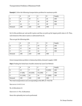
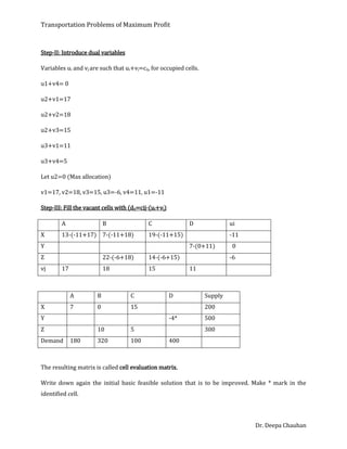
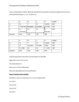
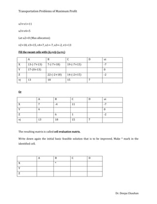
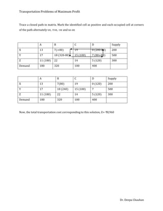
Transportation Problems of Maximum Profit
Dr. Deepa Chauhan
Transportation Problems
Maximum Profit
By
Dr. Deepa Chauhan
Associate Professor,
Applied Science & Humanities Department,
Axis Institute of Technology, Kanpur
Transportation Problems of Maximum Profit
Dr. Deepa Chauhan
Transportation Problems of Maximum Profit
The transportation problem may involve maximization of profit rather than minimization of cost.
Such a problem may be solved in one of the following ways:
(a) As maximization of a function is equivalent to minimization of negative of that function, the
given problem may be converted into a minimization problem by multiplying the profit matrix by
(-1). Minimization of this negative profit matrix by the usual method will be equivalent to the
maximization of the given problem.
(b) It may be converted into a minimization problem, by subtracting all the profits from the highest
profit in the matrix. The problem can then be solved by the usual methods.
(c) It may be solved as a maximization problem itself. However, while finding the initial basic
feasible solution, allocations are to be made in highest profit cells, rather than in lowest cost cells.
Also solution will be optimal when all cell evaluations are non positive (≤0).
Transportation Problems of Maximum Profit
Dr. Deepa Chauhan
Example 1: Solve the following transportation problem for maximum profit:
A B C D Supply
X 12 18 6 25 200
Y 8 7 10 18 500
Z 14 3 11 20 300
Demand 180 320 100 400
Sol. In this problem per unit profit is given and thus we pick up the largest profit value is 25. Thus,
each element of the above matrix is subtracted from 25.
Thus we get the following table
A B C D Supply
X 13 7 19 0 200
Y 17 18 15 7 500
Z 11 22 14 5 300
Demand 180 320 100 400
Given transportation problem is balanced problem, demand=supply=1000
Step-I: Finding the Initial basic feasible solution by Least Cost Method:
A B C D Supply
X 13 7 19 0 (200) 200
Y 17 (80) 18 (320) 15 (100) 7 500
Z 11 (100) 22 14 5 (200) 300
Demand 180 320 100 400
The total transportation cost corresponding to this BFS, Z= ₹10,720
Here m+n-1=4+3-1=6
No. of allocations=6
Since m+n-1= No. of allocations
Hence the optimality test can be performed.
Transportation Problems of Maximum Profit
Dr. Deepa Chauhan
Step-II: Introduce dual variables
Variables ui and vj are such that ui+vj=cij, for occupied cells.
u1+v4= 0
u2+v1=17
u2+v2=18
u2+v3=15
u3+v1=11
u3+v4=5
Let u2=0 (Max allocation)
v1=17, v2=18, v3=15, u3=-6, v4=11, u1=-11
Step-III: Fill the vacant cells with (dij=cij-(ui+vj)
A B C D ui
X 13-(-11+17) 7-(-11+18) 19-(-11+15) -11
Y 7-(0+11) 0
Z 22-(-6+18) 14-(-6+15) -6
vj 17 18 15 11
A B C D Supply
X 7 0 15 200
Y -4* 500
Z 10 5 300
Demand 180 320 100 400
The resulting matrix is called cell evaluation matrix.
Write down again the initial basic feasible solution that is to be improved. Make * mark in the
identified cell.
Transportation Problems of Maximum Profit
Dr. Deepa Chauhan
Trace a closed path in matrix. Mark the identified cell as positive and each occupied cell at corners
of the path alternately-ve, +ve, -ve and so on
A B C D Supply
X 13 7 19 0 (200) 200
Y 17 (80-80) 18 (320) 15 (100) *7(+80) 500
Z 11
(100+80)
22 14 5
(200-80)
300
Demand 180 320 100 400
A B C D Supply
X 13 7 19 0 (200) 200
Y 17 18 (320) 15 (100) 7(80) 500
Z 11 (180) 22 14 5 (120) 300
Demand 180 320 100 400
Total transportation cost of the current solution: Z=₹10,400
Again, Here m+n-1=4+3-1=6
No. of allocations=6
Since m+n-1= No. of allocations
Hence the optimality test can be performed.
Step-II: Introduce dual variables
Variables ui and vj are such that ui+vj=cij, for occupied cells.
u1+v4=0
u2+v2=18
u2+v3=15
u2+v4=7
Transportation Problems of Maximum Profit
Dr. Deepa Chauhan
u3+v1=11
u3+v4=5
Let u2=0 (Max allocation)
v2=18, v3=15, v4=7, u1=-7, u3=-2, v1=13
Fill the vacant cells with (dij=cij-(ui+vj)
A B C D ui
X 13-(-7+13) 7-(-7+18) 19-(-7+15) -7
Y 17-(0+13) 0
Z 22-(-2+18) 14-(-2+15) -2
vj 13 18 15 7
Or
A B C D ui
X 7 -4 11 -7
Y 4 0
Z 6 1 -2
vj 13 18 15 7
The resulting matrix is called cell evaluation matrix.
Write down again the initial basic feasible solution that is to be improved. Make * mark in the
identified cell.
A B C D
X *
Y
Z
Transportation Problems of Maximum Profit
Dr. Deepa Chauhan
Trace a closed path in matrix. Mark the identified cell as positive and each occupied cell at corners
of the path alternately-ve, +ve, -ve and so on
A B C D Supply
X 13 7(+80) 19 0 (200-80) 200
Y 17 18 (320-80) 15 (100) 7 (80+80) 500
Z 11 (180) 22 14 5 (120) 300
Demand 180 320 100 400
A B C D Supply
X 13 7(80) 19 0 (120) 200
Y 17 18 (240) 15 (100) 7 500
Z 11 (180) 22 14 5 (120) 300
Demand 180 320 100 400
Now, the total transportation cost corresponding to this solution, Z= ₹8,960

Transportation Problems-Maximum Profit

  • 1.
    Transportation Problems ofMaximum Profit Dr. Deepa Chauhan Transportation Problems Maximum Profit By Dr. Deepa Chauhan Associate Professor, Applied Science & Humanities Department, Axis Institute of Technology, Kanpur
  • 2.
    Transportation Problems ofMaximum Profit Dr. Deepa Chauhan Transportation Problems of Maximum Profit The transportation problem may involve maximization of profit rather than minimization of cost. Such a problem may be solved in one of the following ways: (a) As maximization of a function is equivalent to minimization of negative of that function, the given problem may be converted into a minimization problem by multiplying the profit matrix by (-1). Minimization of this negative profit matrix by the usual method will be equivalent to the maximization of the given problem. (b) It may be converted into a minimization problem, by subtracting all the profits from the highest profit in the matrix. The problem can then be solved by the usual methods. (c) It may be solved as a maximization problem itself. However, while finding the initial basic feasible solution, allocations are to be made in highest profit cells, rather than in lowest cost cells. Also solution will be optimal when all cell evaluations are non positive (≤0).
  • 3.
    Transportation Problems ofMaximum Profit Dr. Deepa Chauhan Example 1: Solve the following transportation problem for maximum profit: A B C D Supply X 12 18 6 25 200 Y 8 7 10 18 500 Z 14 3 11 20 300 Demand 180 320 100 400 Sol. In this problem per unit profit is given and thus we pick up the largest profit value is 25. Thus, each element of the above matrix is subtracted from 25. Thus we get the following table A B C D Supply X 13 7 19 0 200 Y 17 18 15 7 500 Z 11 22 14 5 300 Demand 180 320 100 400 Given transportation problem is balanced problem, demand=supply=1000 Step-I: Finding the Initial basic feasible solution by Least Cost Method: A B C D Supply X 13 7 19 0 (200) 200 Y 17 (80) 18 (320) 15 (100) 7 500 Z 11 (100) 22 14 5 (200) 300 Demand 180 320 100 400 The total transportation cost corresponding to this BFS, Z= ₹10,720 Here m+n-1=4+3-1=6 No. of allocations=6 Since m+n-1= No. of allocations Hence the optimality test can be performed.
  • 4.
    Transportation Problems ofMaximum Profit Dr. Deepa Chauhan Step-II: Introduce dual variables Variables ui and vj are such that ui+vj=cij, for occupied cells. u1+v4= 0 u2+v1=17 u2+v2=18 u2+v3=15 u3+v1=11 u3+v4=5 Let u2=0 (Max allocation) v1=17, v2=18, v3=15, u3=-6, v4=11, u1=-11 Step-III: Fill the vacant cells with (dij=cij-(ui+vj) A B C D ui X 13-(-11+17) 7-(-11+18) 19-(-11+15) -11 Y 7-(0+11) 0 Z 22-(-6+18) 14-(-6+15) -6 vj 17 18 15 11 A B C D Supply X 7 0 15 200 Y -4* 500 Z 10 5 300 Demand 180 320 100 400 The resulting matrix is called cell evaluation matrix. Write down again the initial basic feasible solution that is to be improved. Make * mark in the identified cell.
  • 5.
    Transportation Problems ofMaximum Profit Dr. Deepa Chauhan Trace a closed path in matrix. Mark the identified cell as positive and each occupied cell at corners of the path alternately-ve, +ve, -ve and so on A B C D Supply X 13 7 19 0 (200) 200 Y 17 (80-80) 18 (320) 15 (100) *7(+80) 500 Z 11 (100+80) 22 14 5 (200-80) 300 Demand 180 320 100 400 A B C D Supply X 13 7 19 0 (200) 200 Y 17 18 (320) 15 (100) 7(80) 500 Z 11 (180) 22 14 5 (120) 300 Demand 180 320 100 400 Total transportation cost of the current solution: Z=₹10,400 Again, Here m+n-1=4+3-1=6 No. of allocations=6 Since m+n-1= No. of allocations Hence the optimality test can be performed. Step-II: Introduce dual variables Variables ui and vj are such that ui+vj=cij, for occupied cells. u1+v4=0 u2+v2=18 u2+v3=15 u2+v4=7
  • 6.
    Transportation Problems ofMaximum Profit Dr. Deepa Chauhan u3+v1=11 u3+v4=5 Let u2=0 (Max allocation) v2=18, v3=15, v4=7, u1=-7, u3=-2, v1=13 Fill the vacant cells with (dij=cij-(ui+vj) A B C D ui X 13-(-7+13) 7-(-7+18) 19-(-7+15) -7 Y 17-(0+13) 0 Z 22-(-2+18) 14-(-2+15) -2 vj 13 18 15 7 Or A B C D ui X 7 -4 11 -7 Y 4 0 Z 6 1 -2 vj 13 18 15 7 The resulting matrix is called cell evaluation matrix. Write down again the initial basic feasible solution that is to be improved. Make * mark in the identified cell. A B C D X * Y Z
  • 7.
    Transportation Problems ofMaximum Profit Dr. Deepa Chauhan Trace a closed path in matrix. Mark the identified cell as positive and each occupied cell at corners of the path alternately-ve, +ve, -ve and so on A B C D Supply X 13 7(+80) 19 0 (200-80) 200 Y 17 18 (320-80) 15 (100) 7 (80+80) 500 Z 11 (180) 22 14 5 (120) 300 Demand 180 320 100 400 A B C D Supply X 13 7(80) 19 0 (120) 200 Y 17 18 (240) 15 (100) 7 500 Z 11 (180) 22 14 5 (120) 300 Demand 180 320 100 400 Now, the total transportation cost corresponding to this solution, Z= ₹8,960