Download as PDF, PPTX
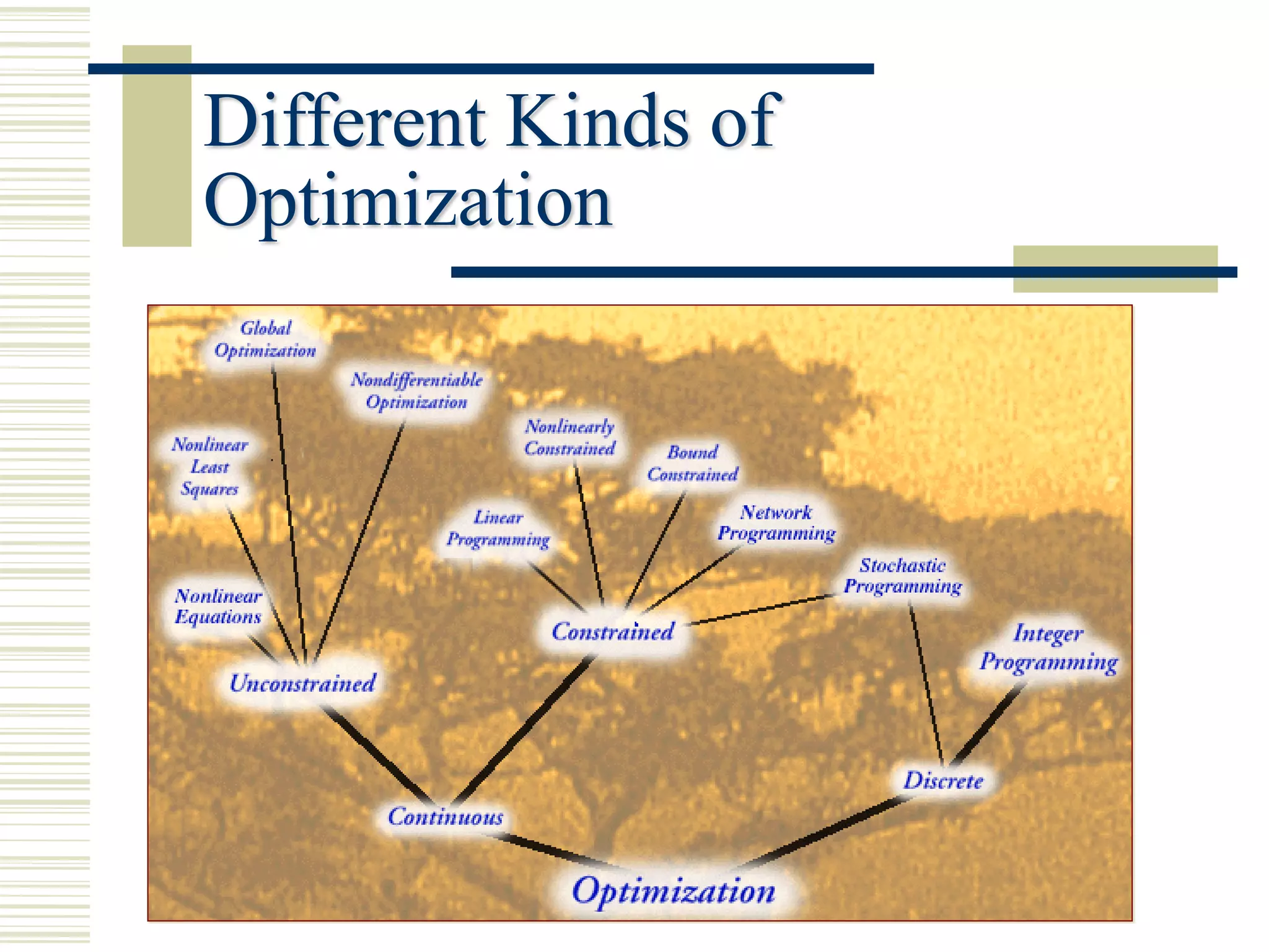

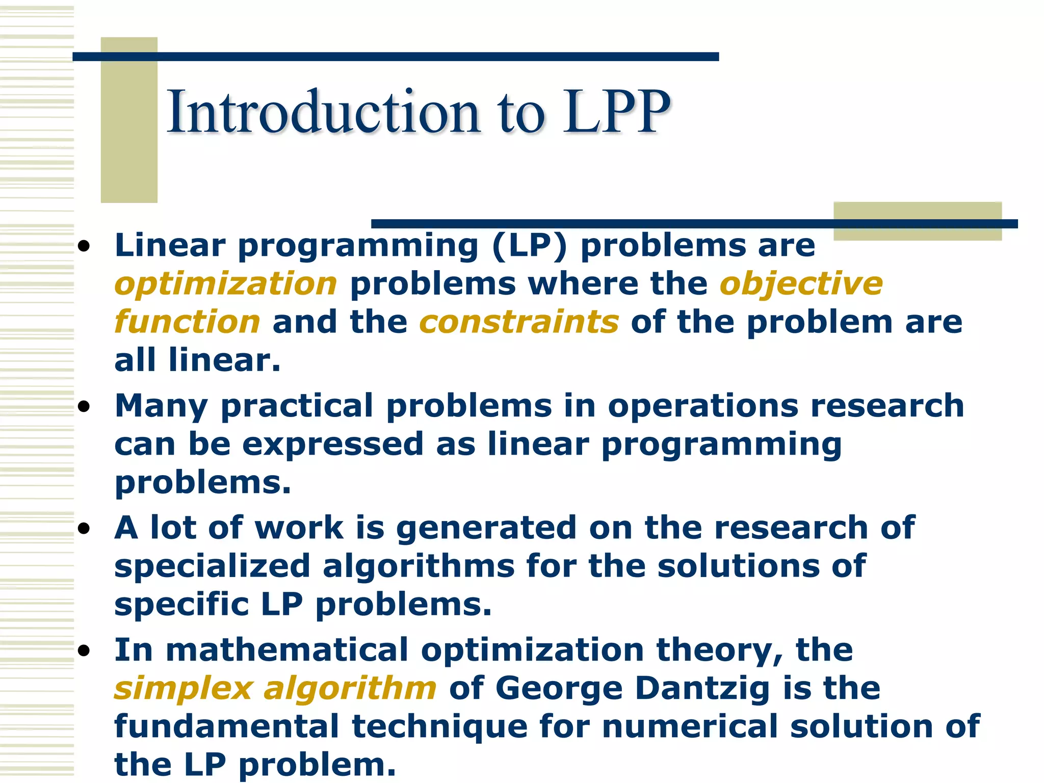


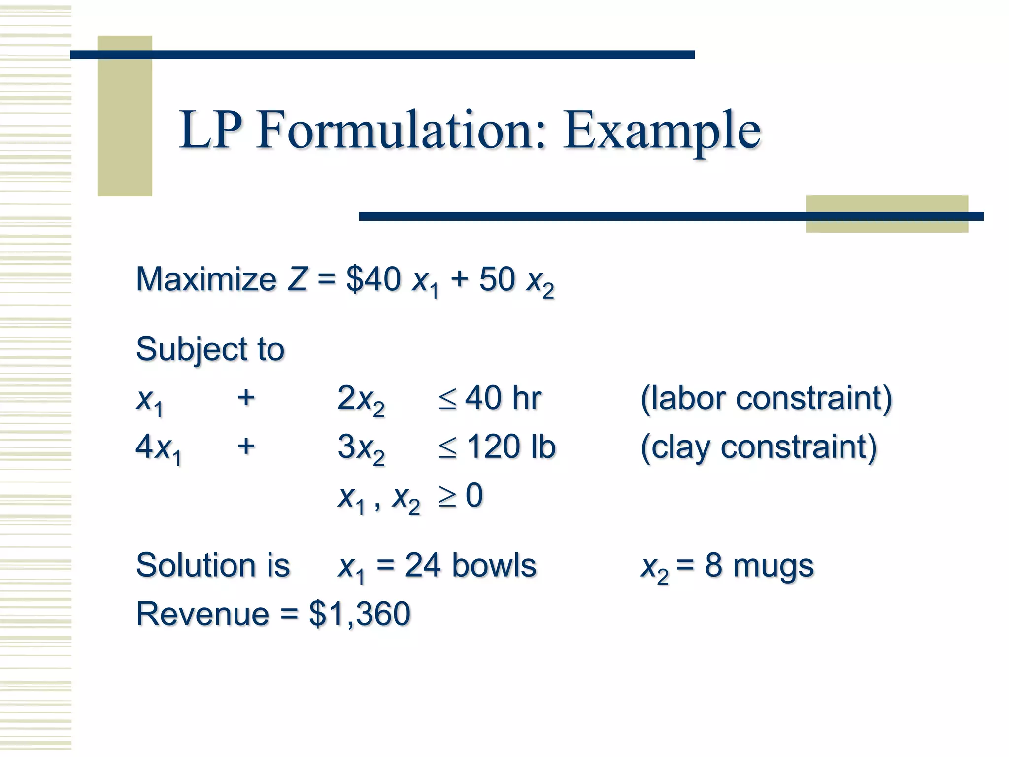
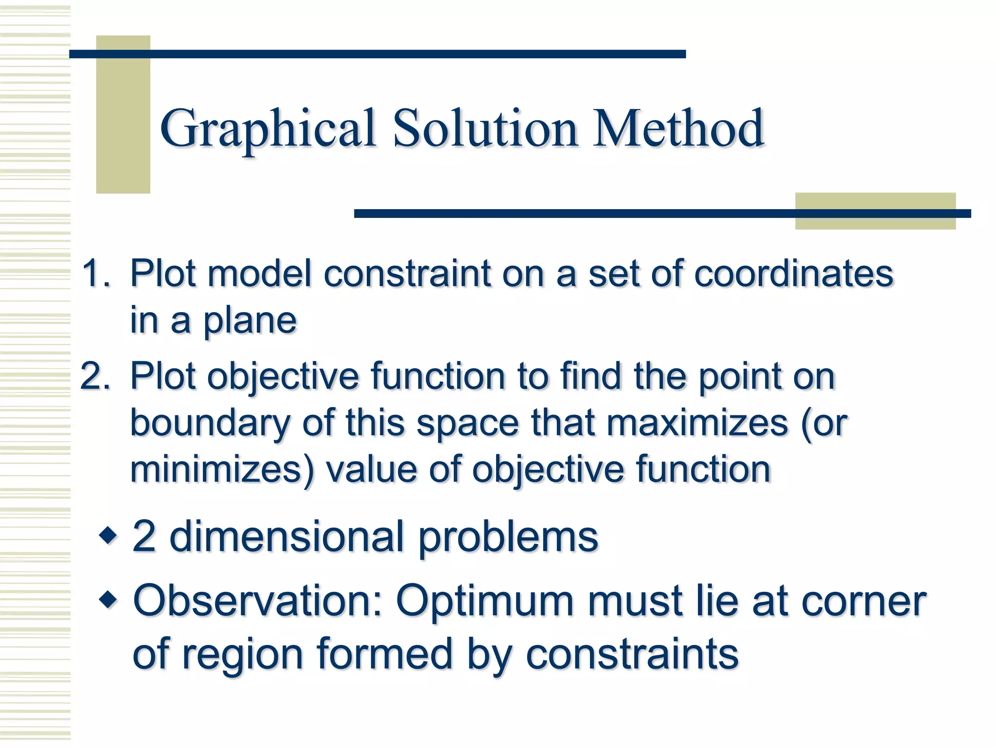

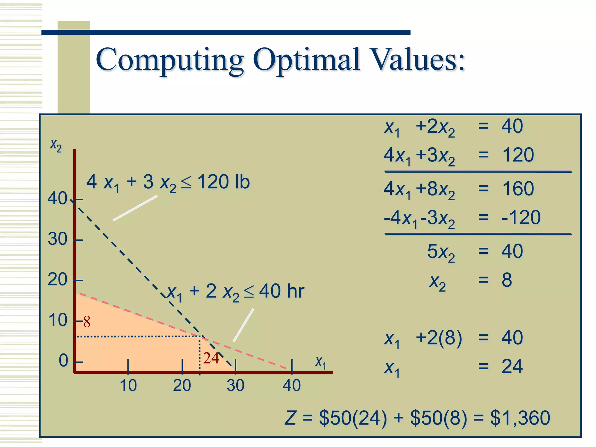


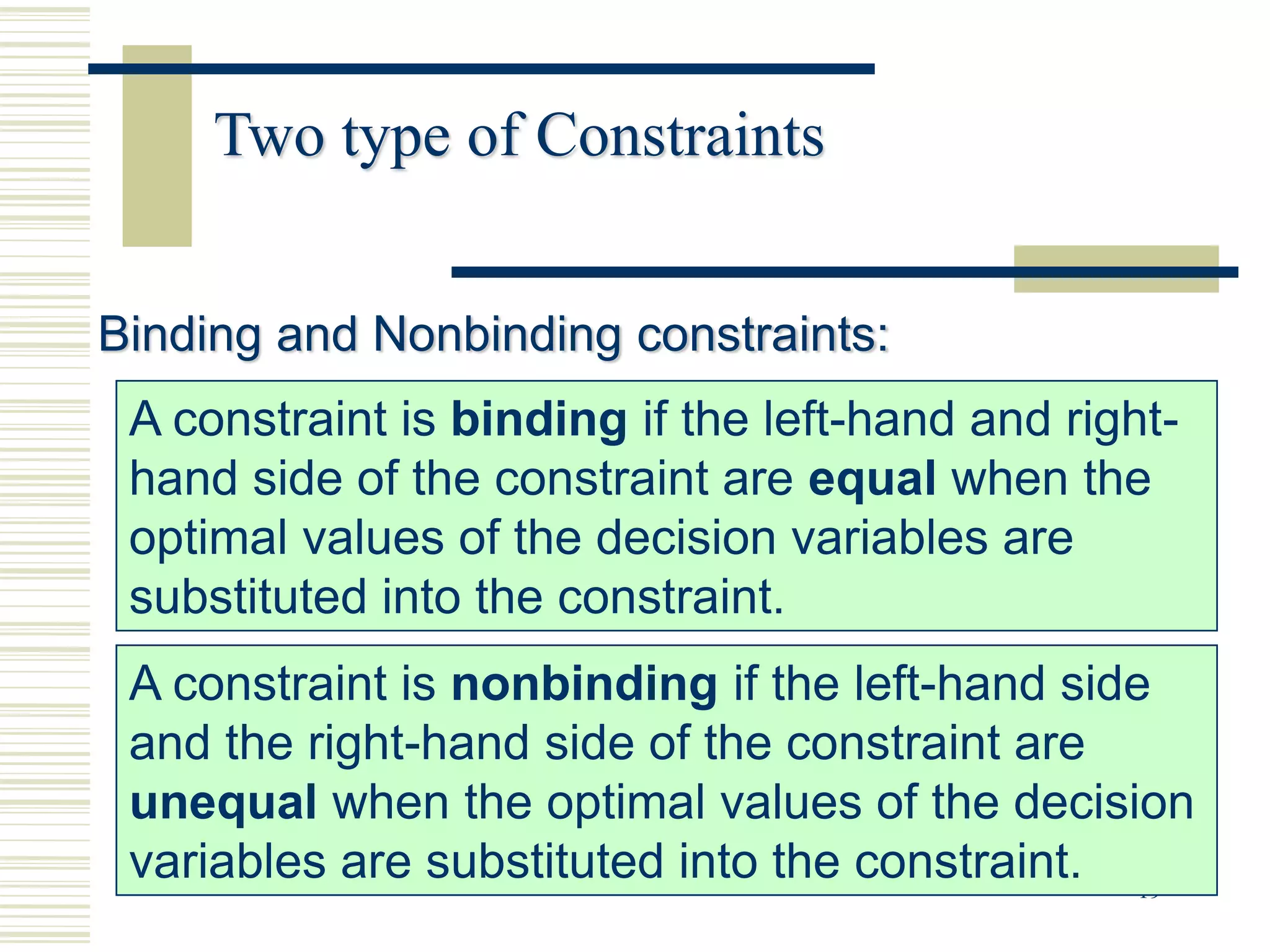


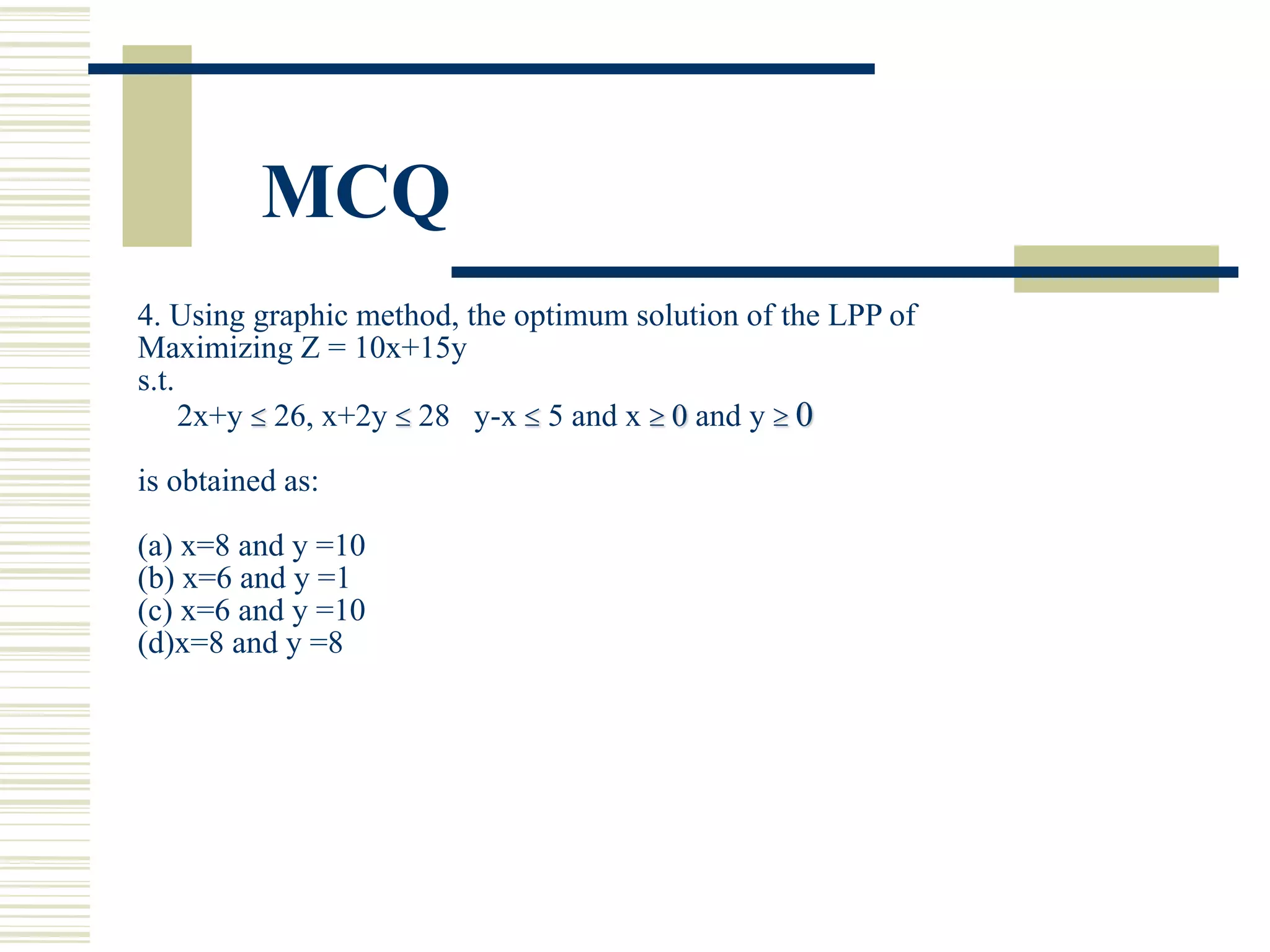


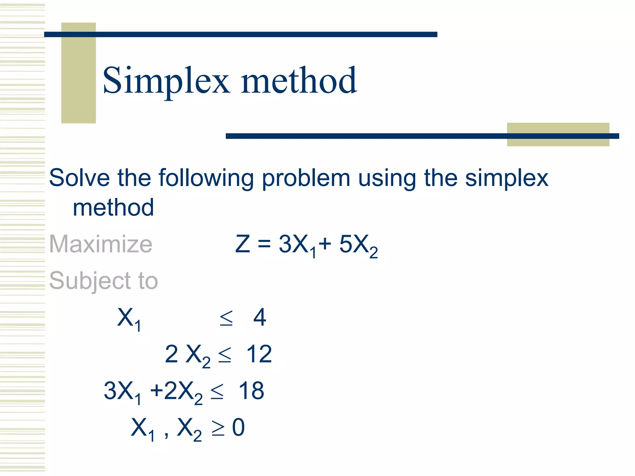


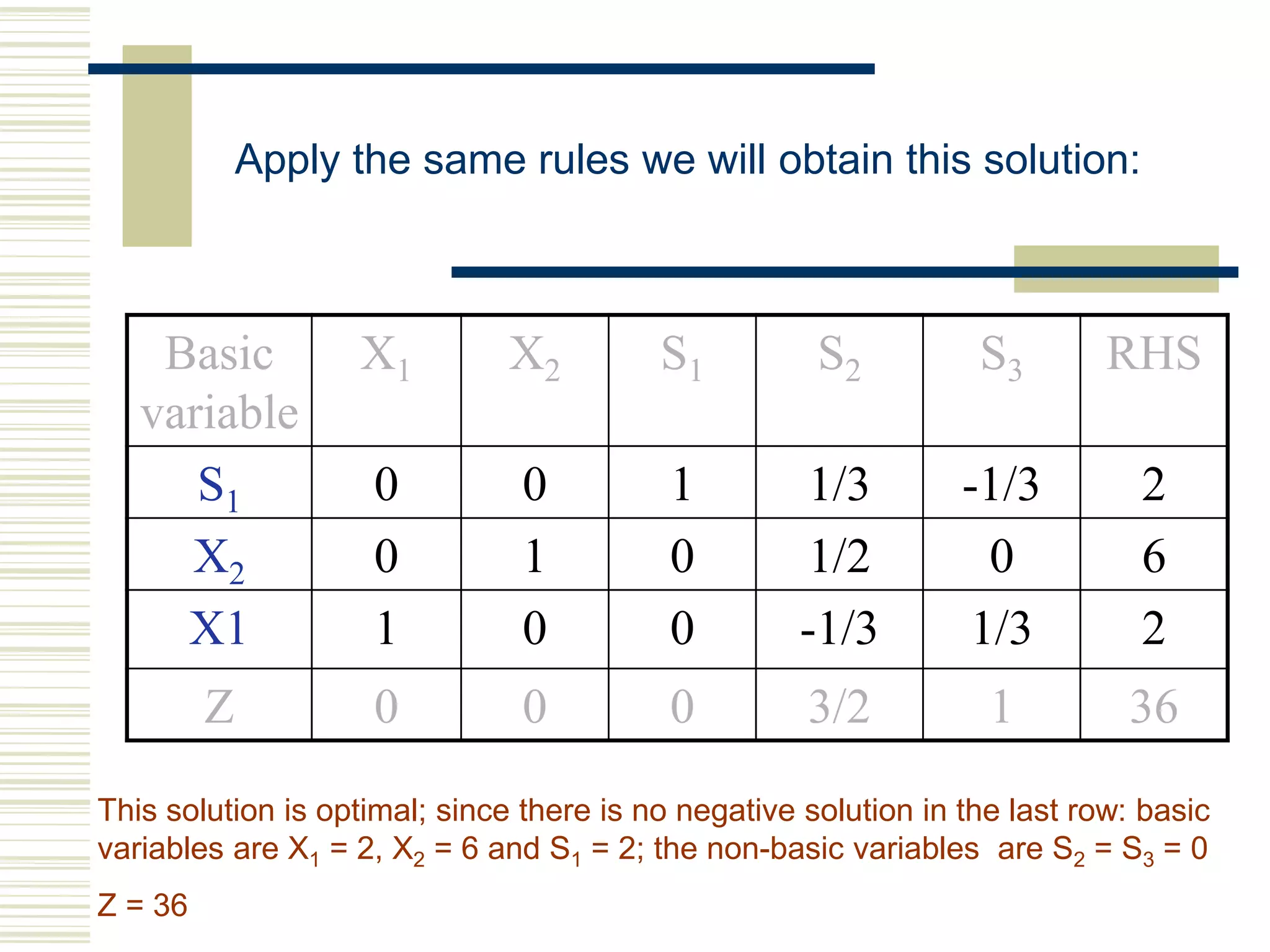


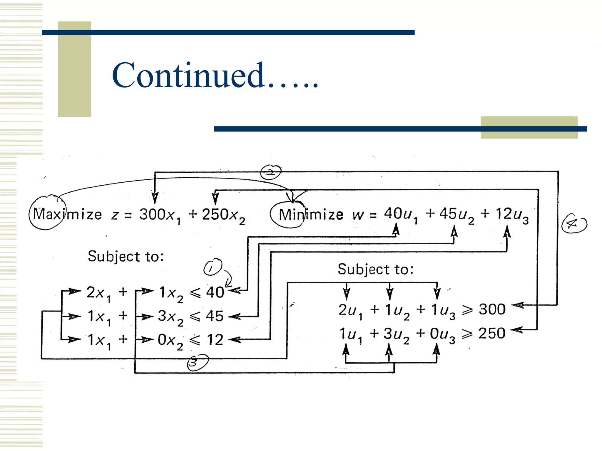


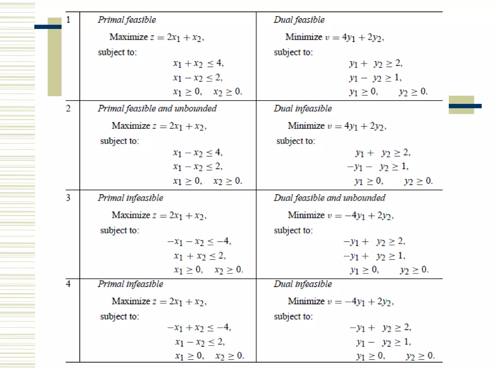


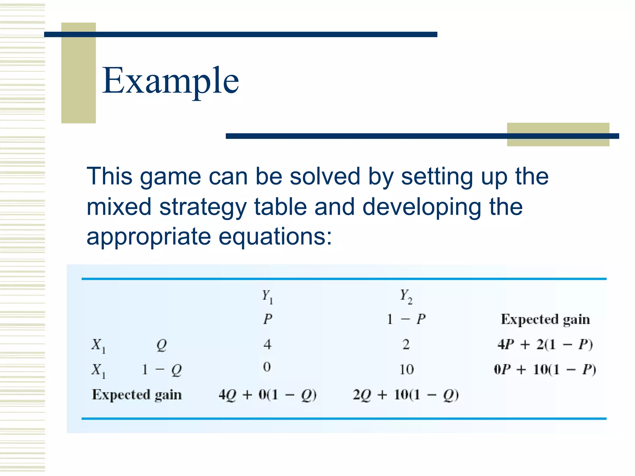
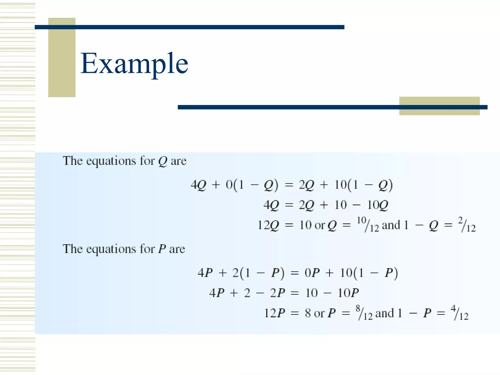


The document provides information about linear programming problems (LPP), including: - LPPs involve optimization of a linear objective function subject to linear constraints. - Graphical and algebraic methods can be used to find the optimal solution, which must occur at a corner point of the feasible region. - The simplex method is an algorithm that moves from one corner point to another to optimize the objective function. - Examples are provided to illustrate LPP formulation, graphical solution, and use of the simplex method to iteratively find an optimal solution.