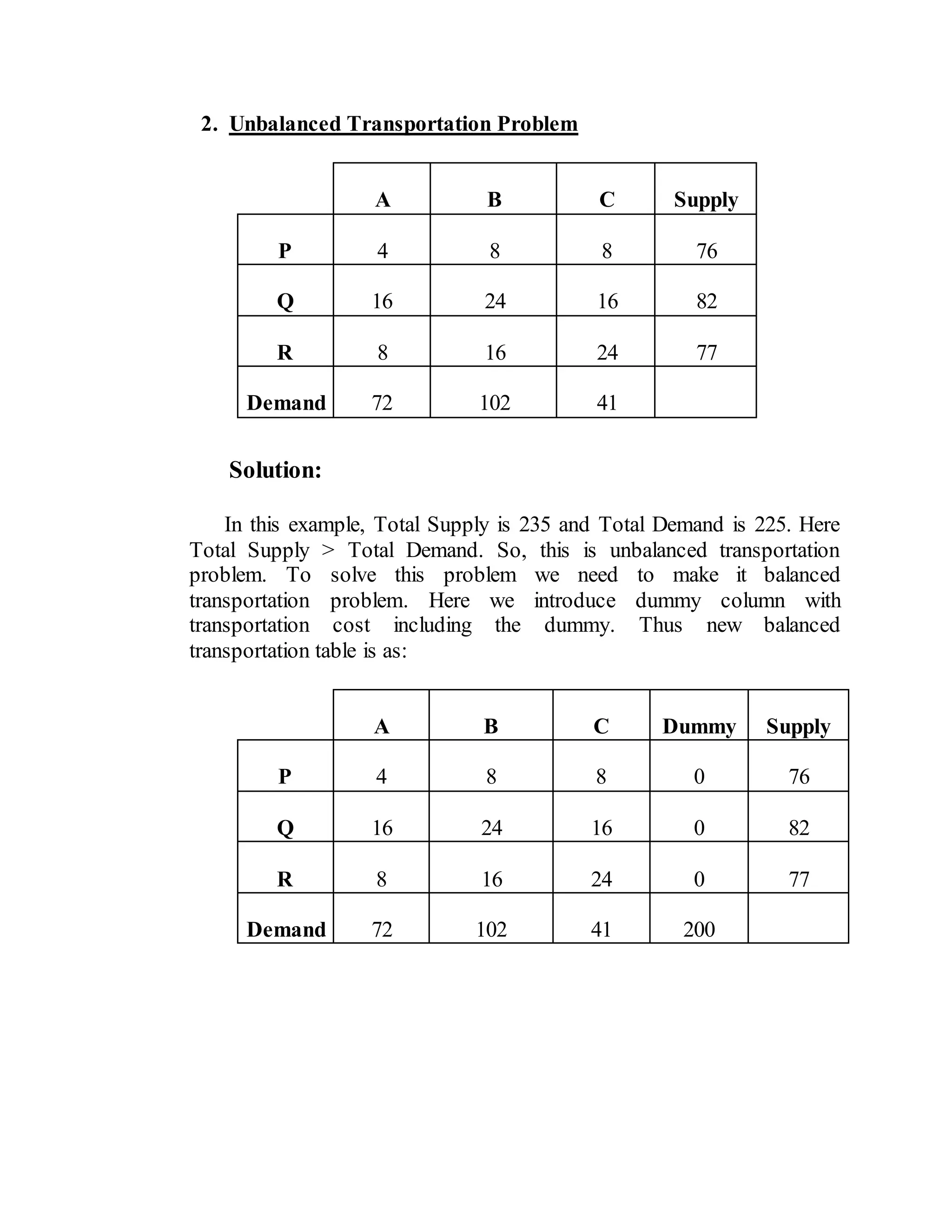
Vogel's Approximation Method (VAM) is a method for solving transportation problems that considers penalties (opportunity costs) associated with not shipping to cells with the lowest costs. It works as follows:
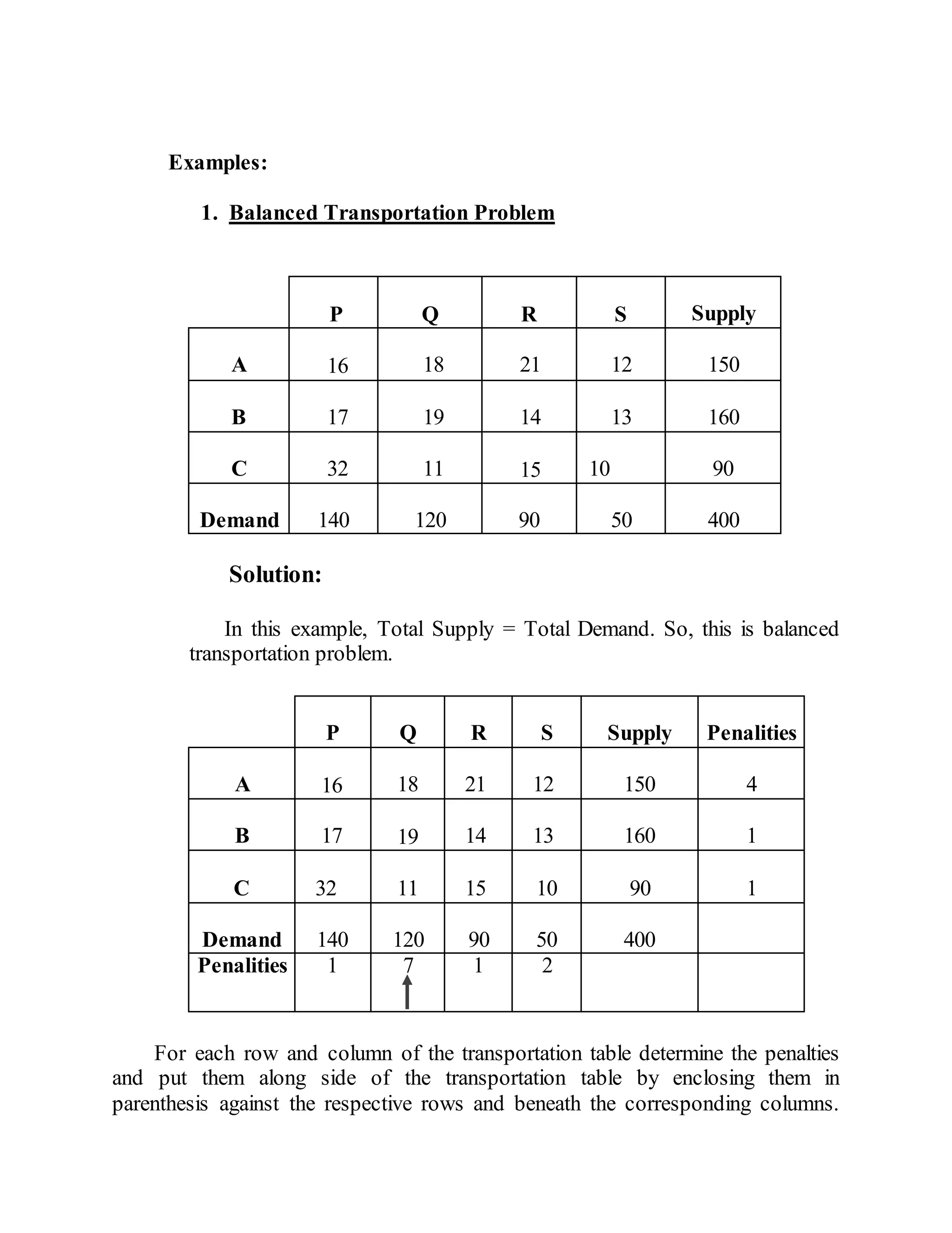
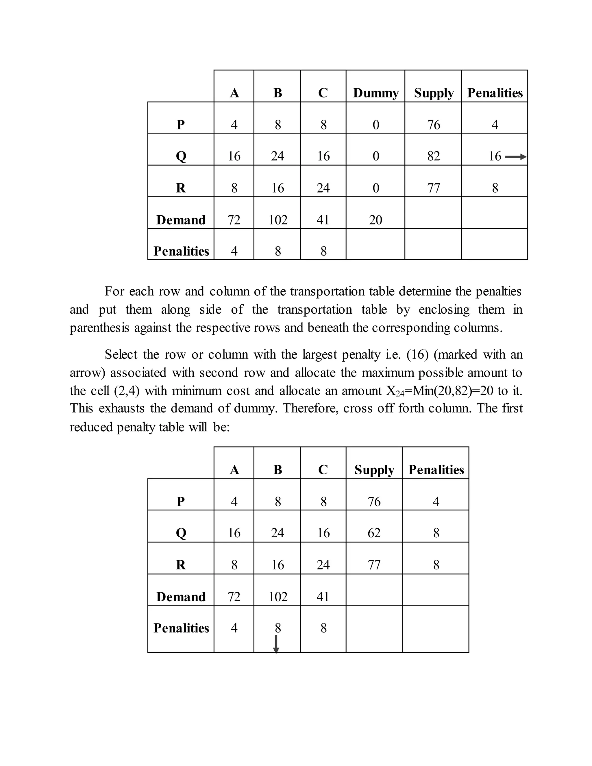
1. Compute penalties for each row and column based on the difference between the lowest and second lowest costs.
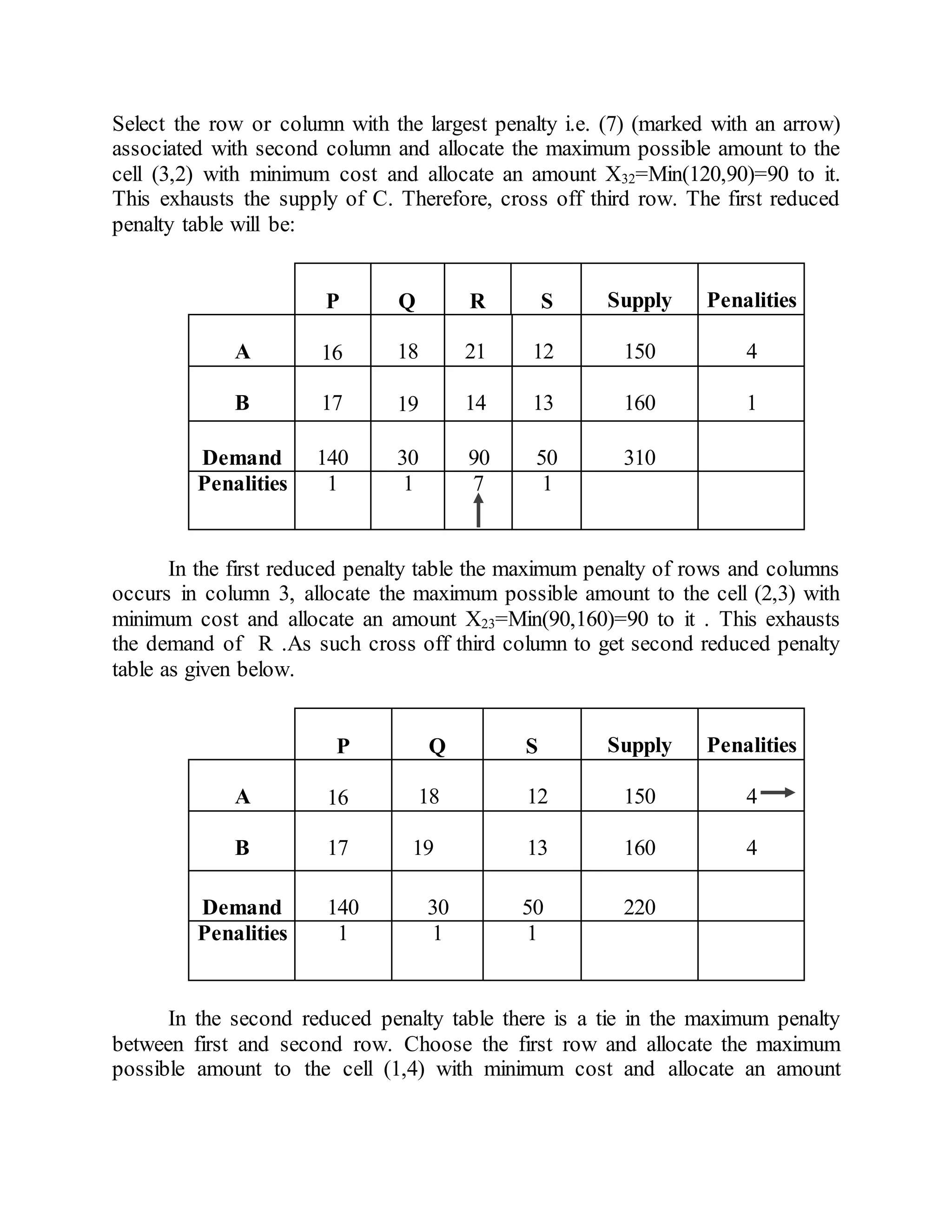
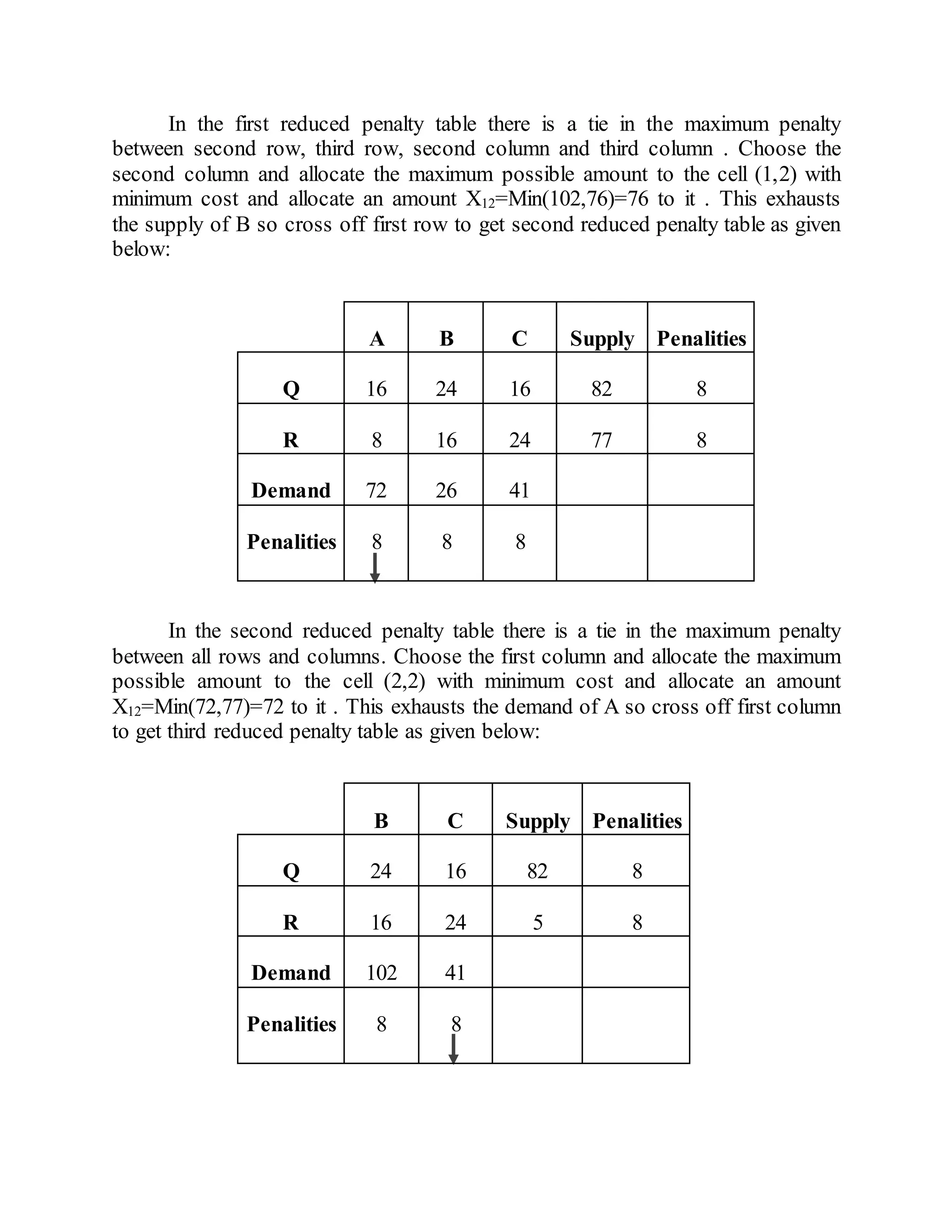
2. Ship to the cell in the row or column with the largest penalty, removing that row or column.
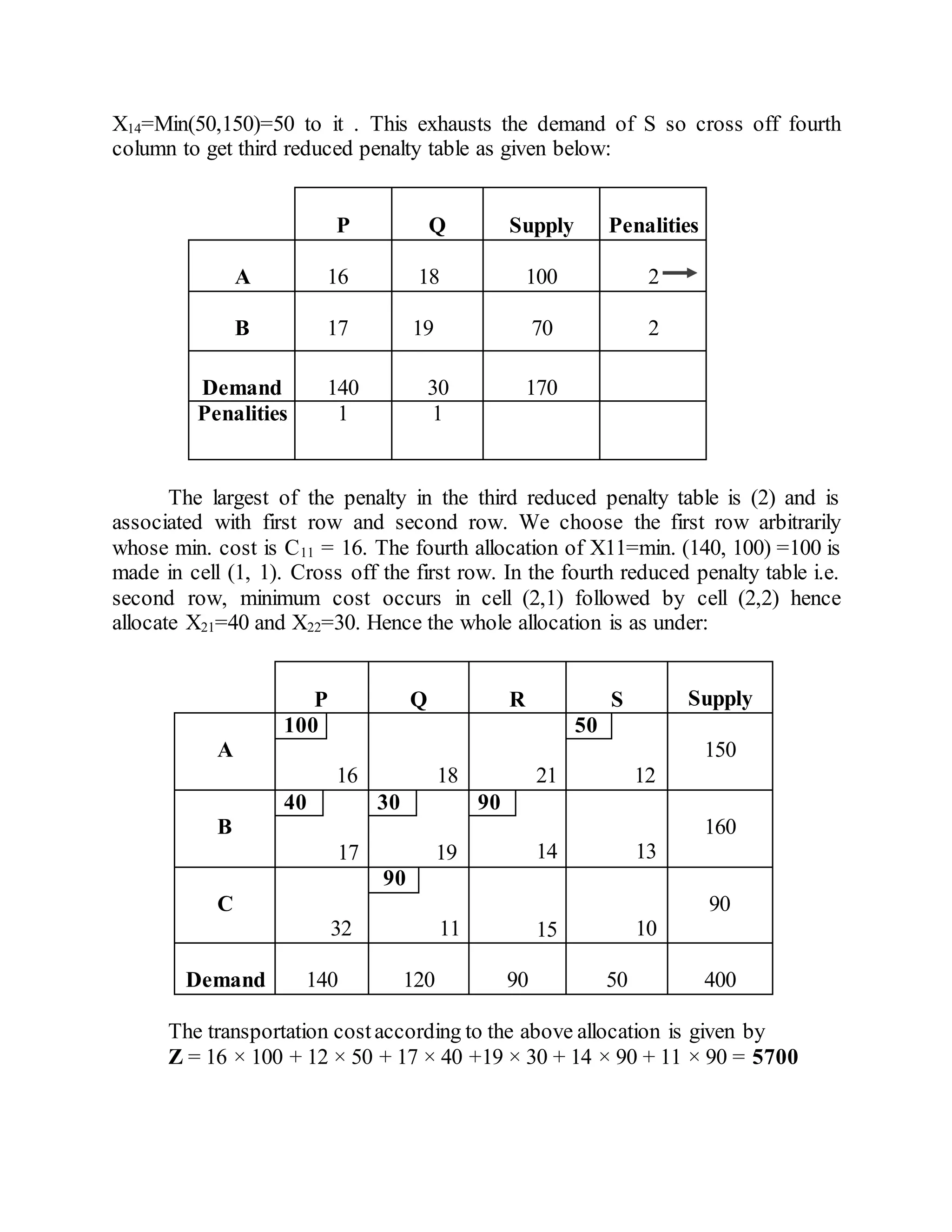
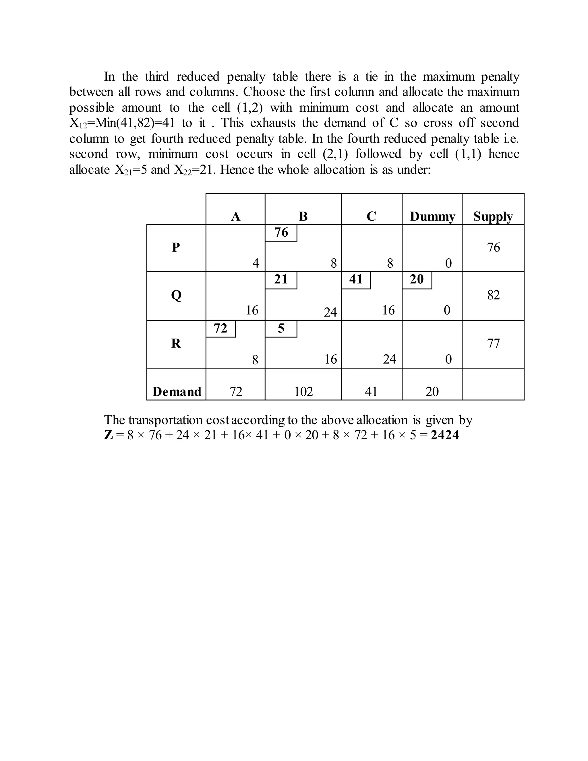
3. Recompute penalties and repeat until all shipments are allocated. VAM finds an initial solution close to optimal with few iterations.