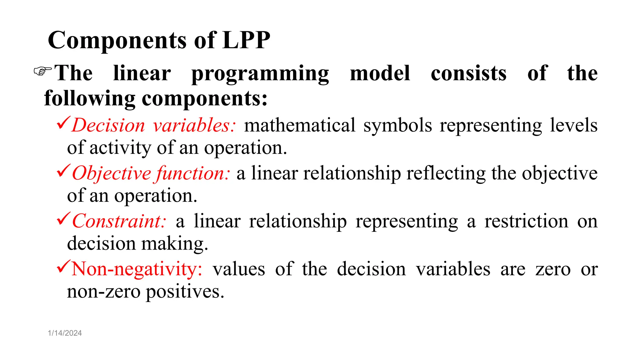
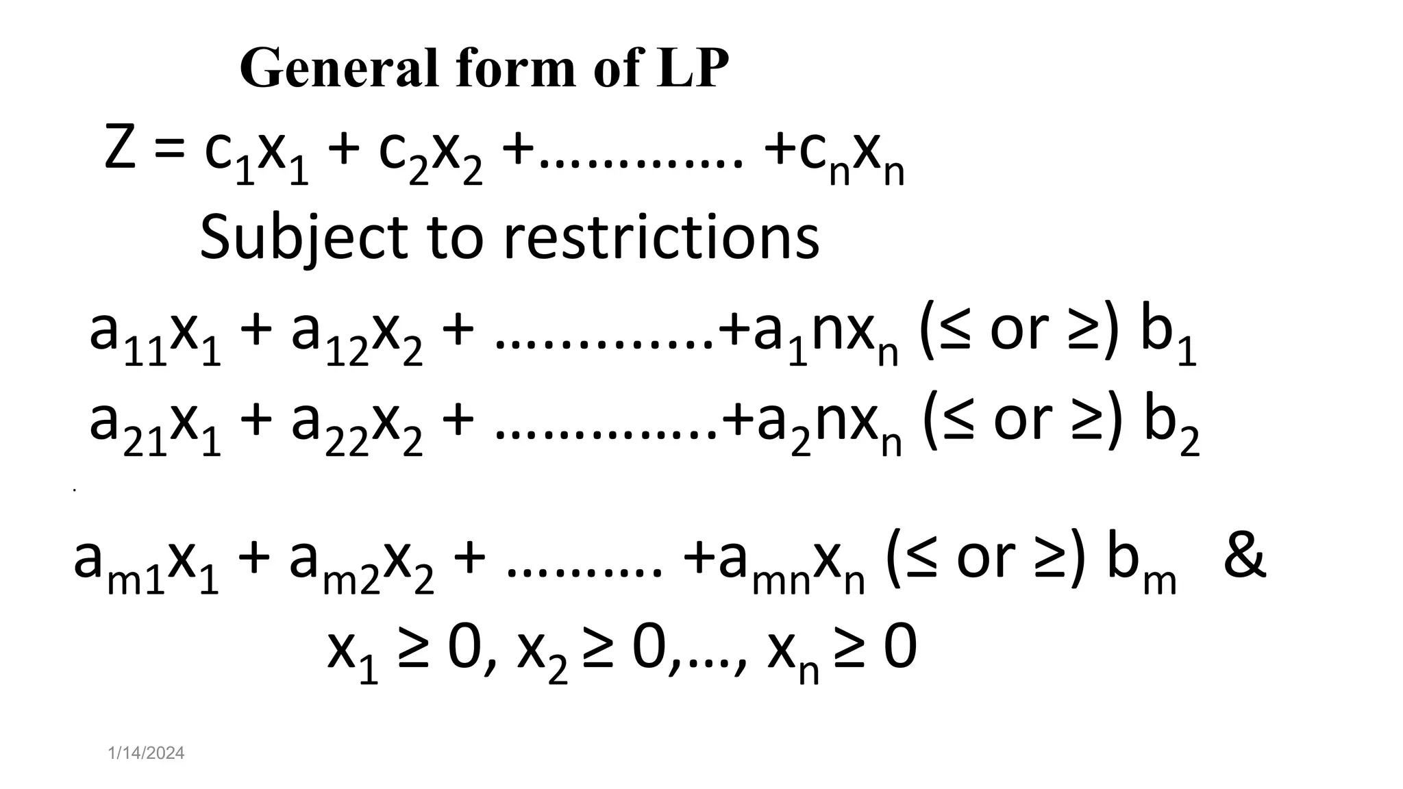
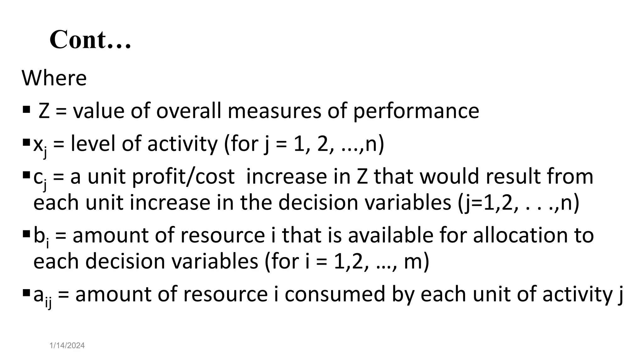
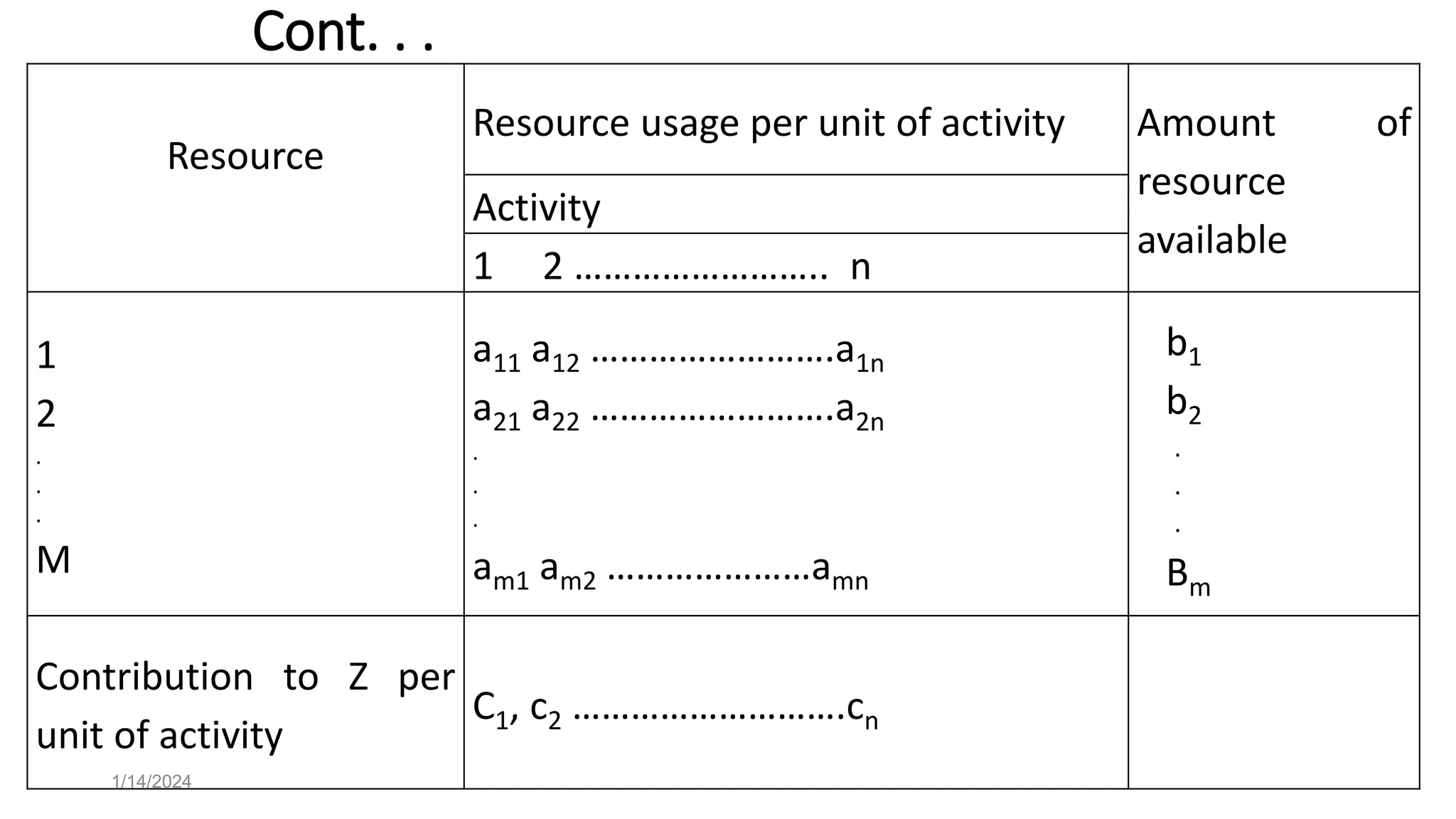
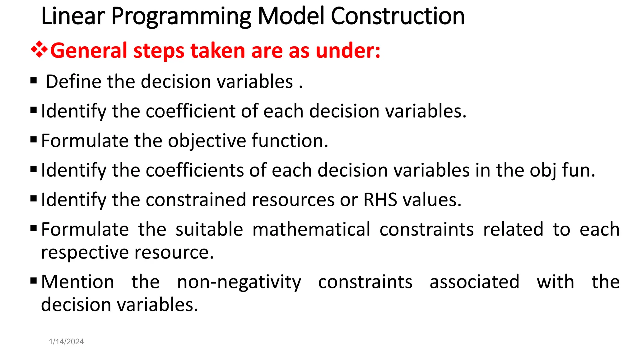
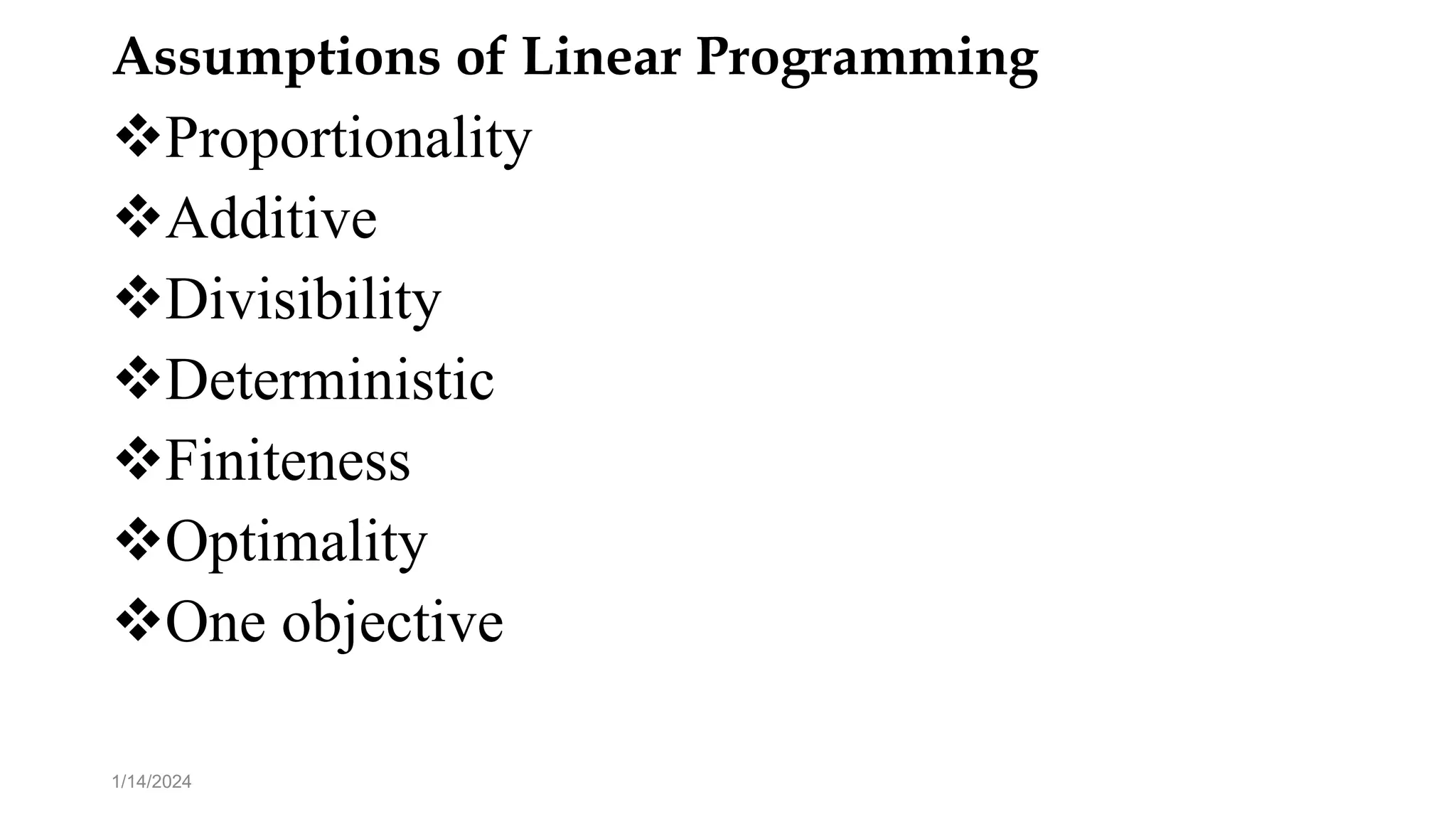
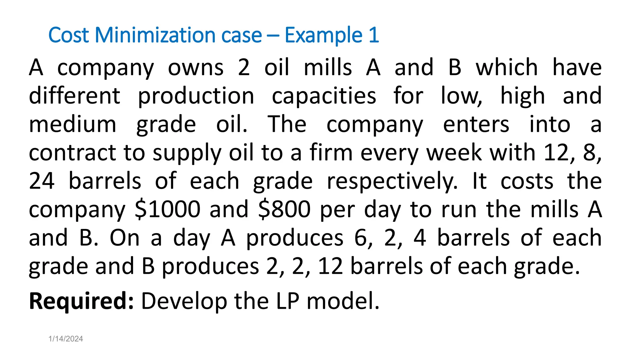
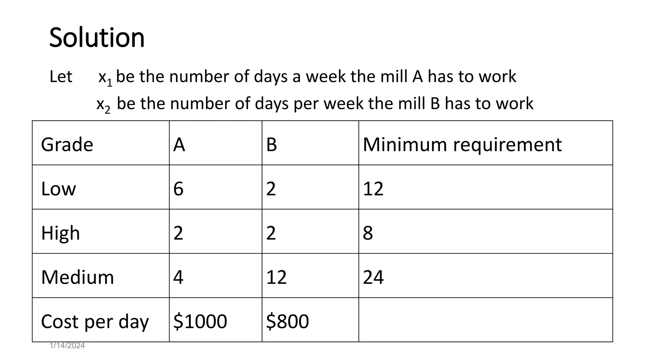
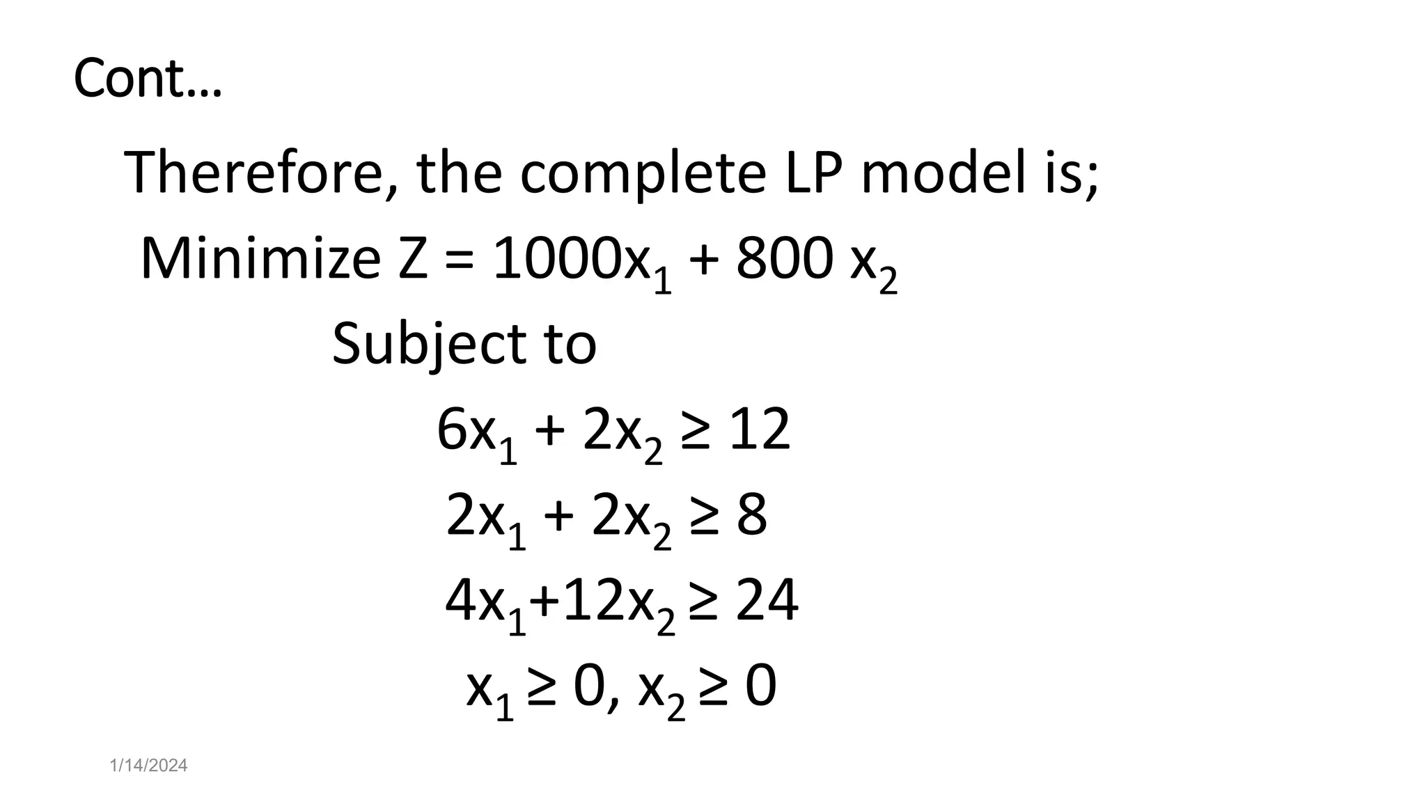
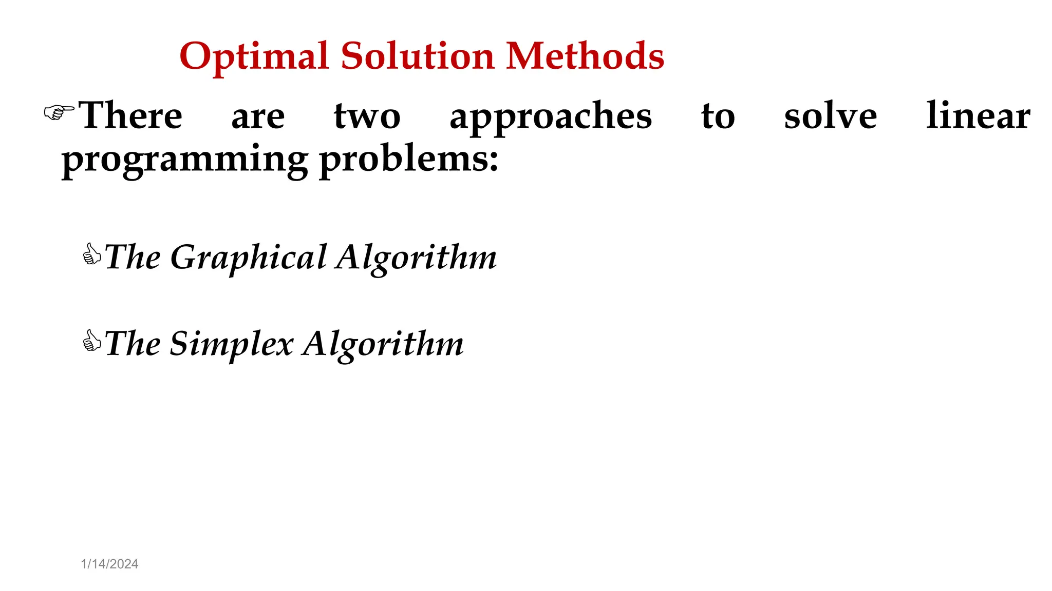
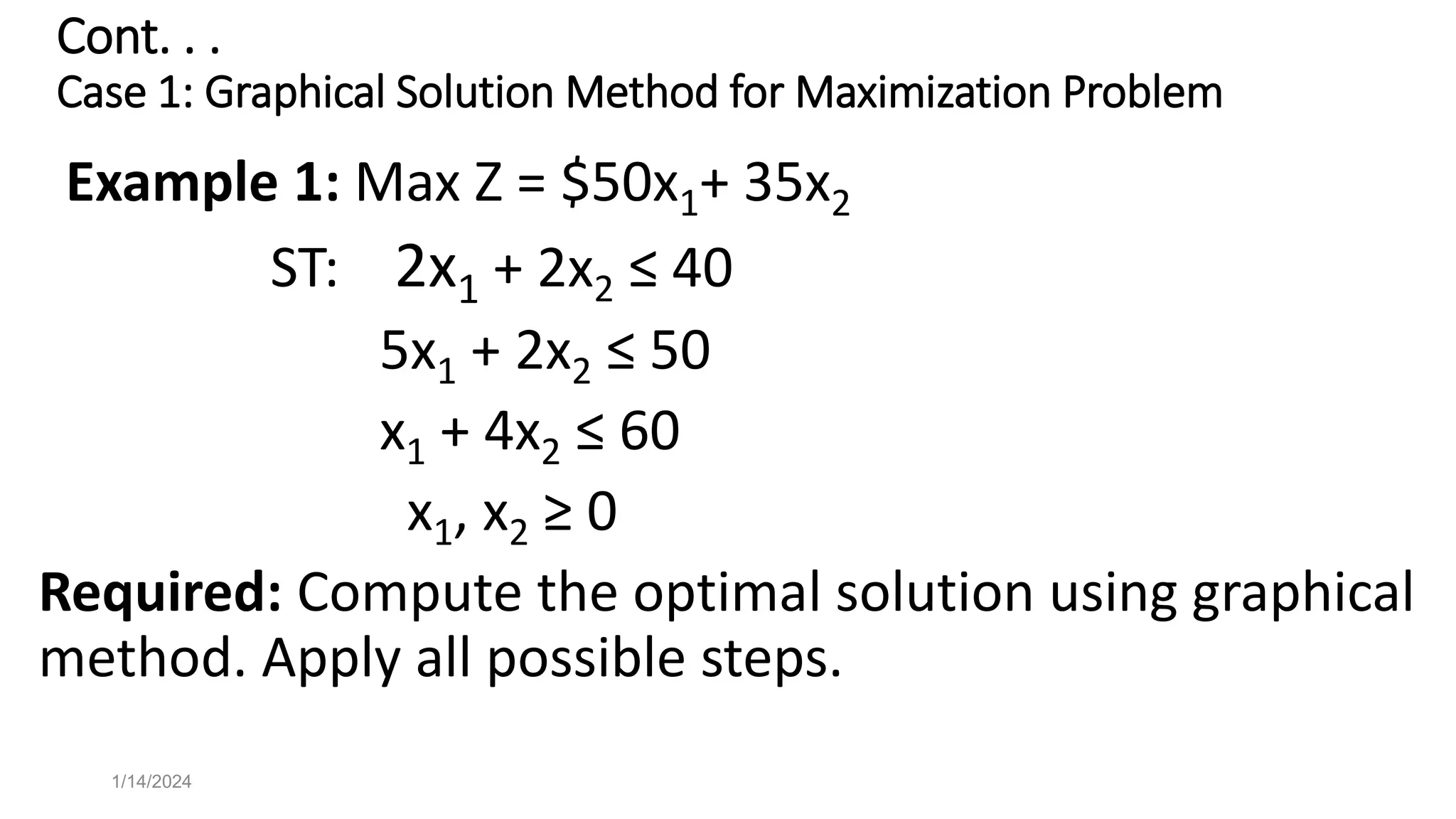
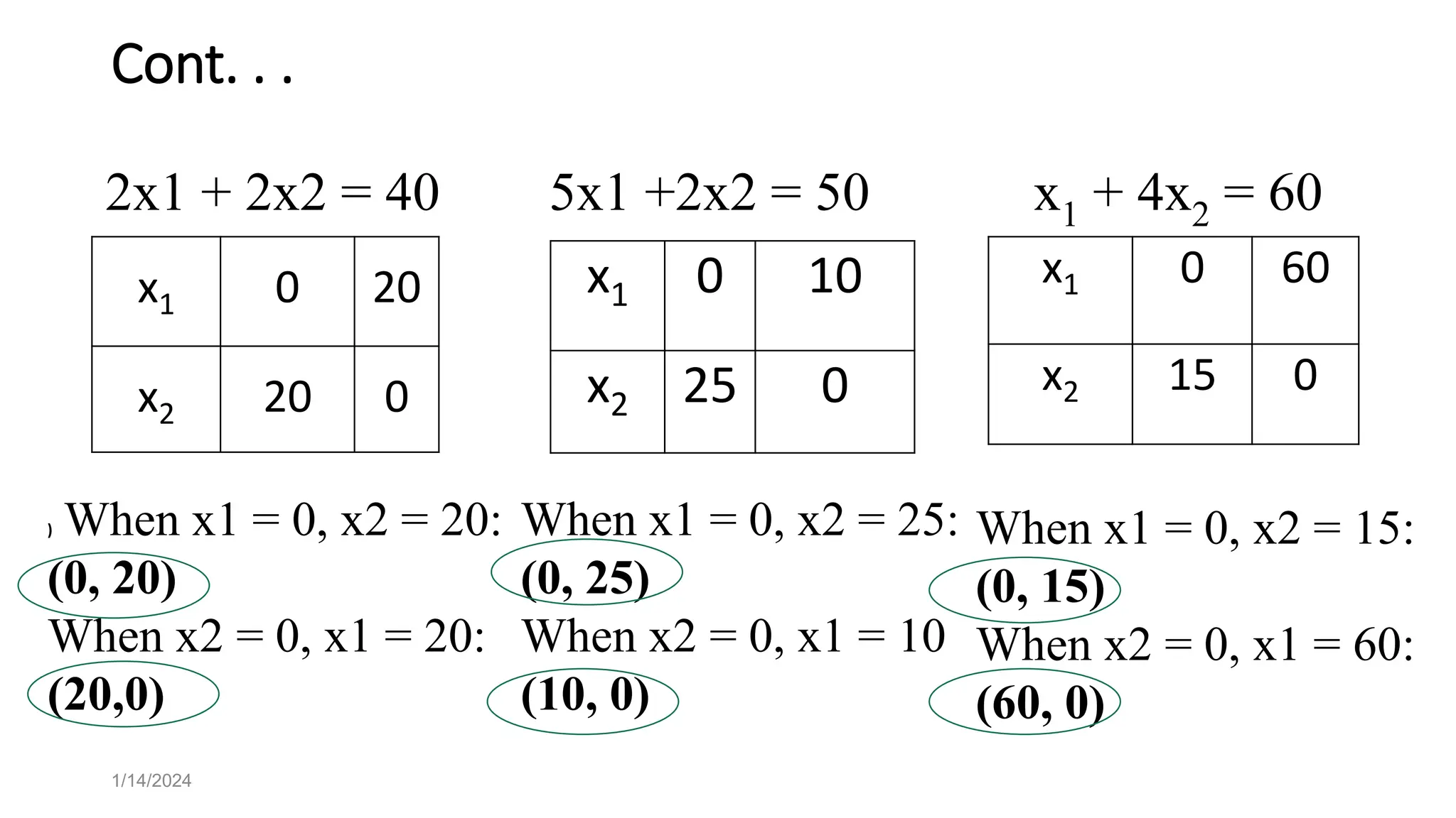
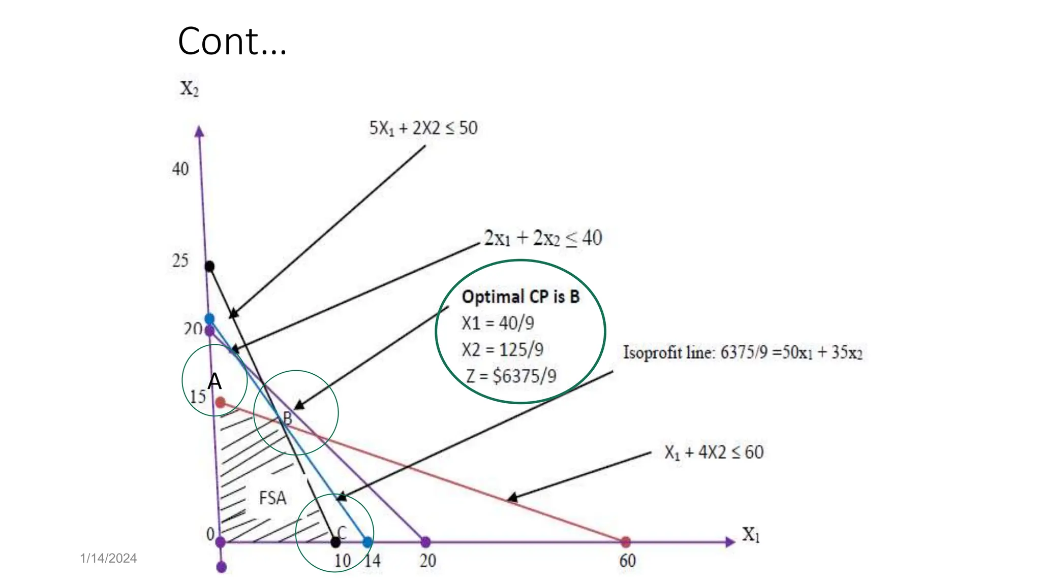
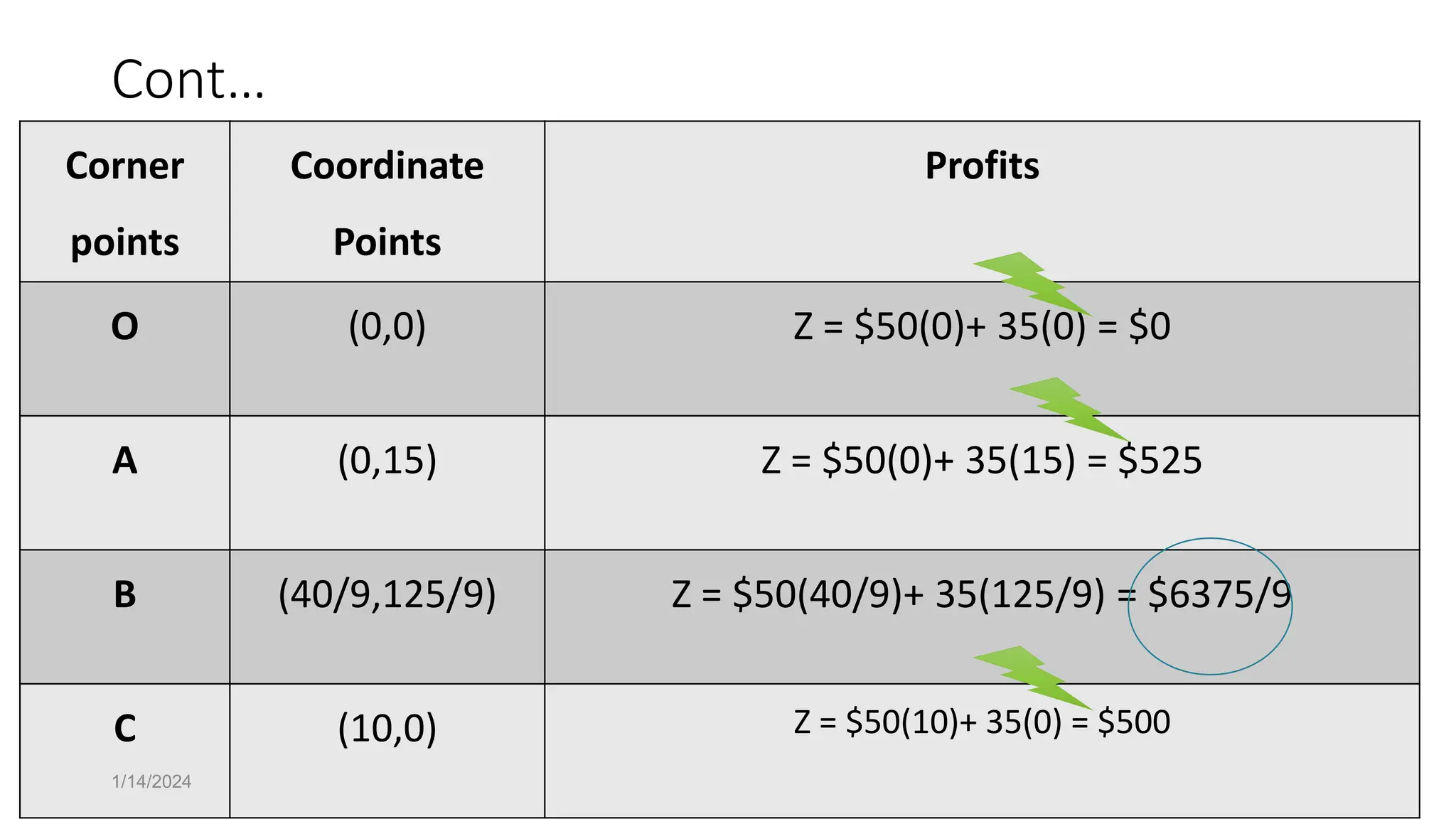
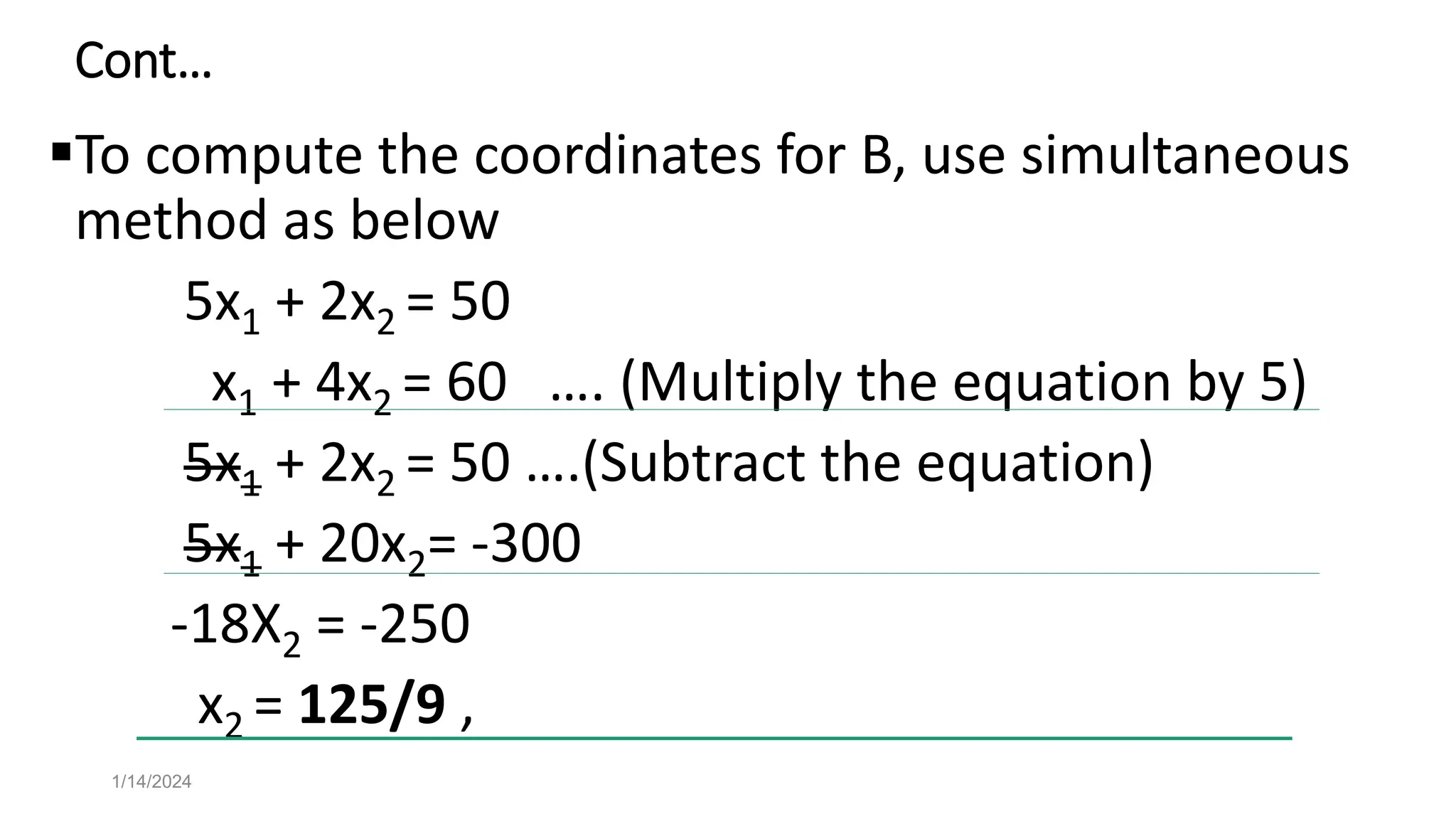
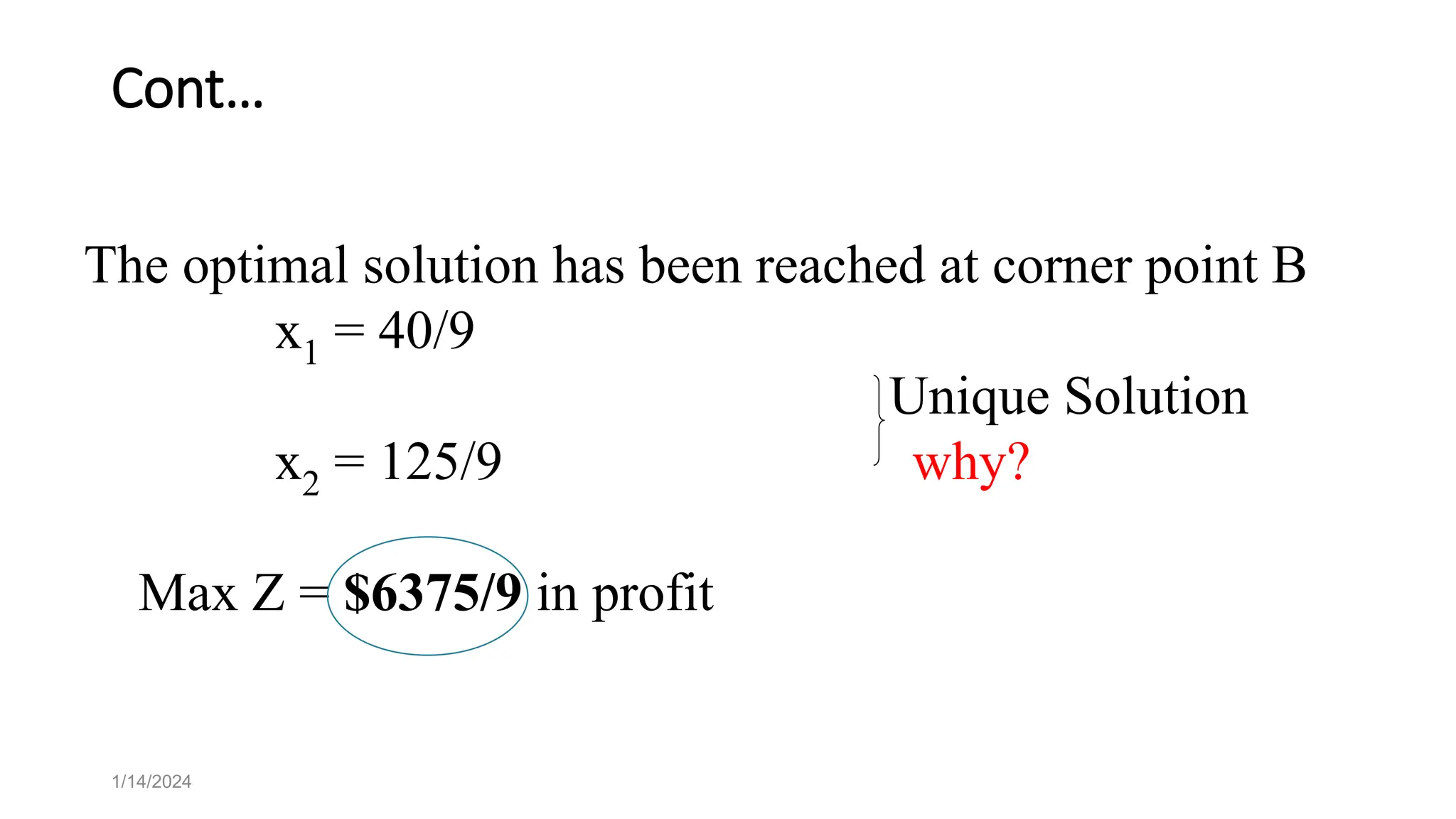
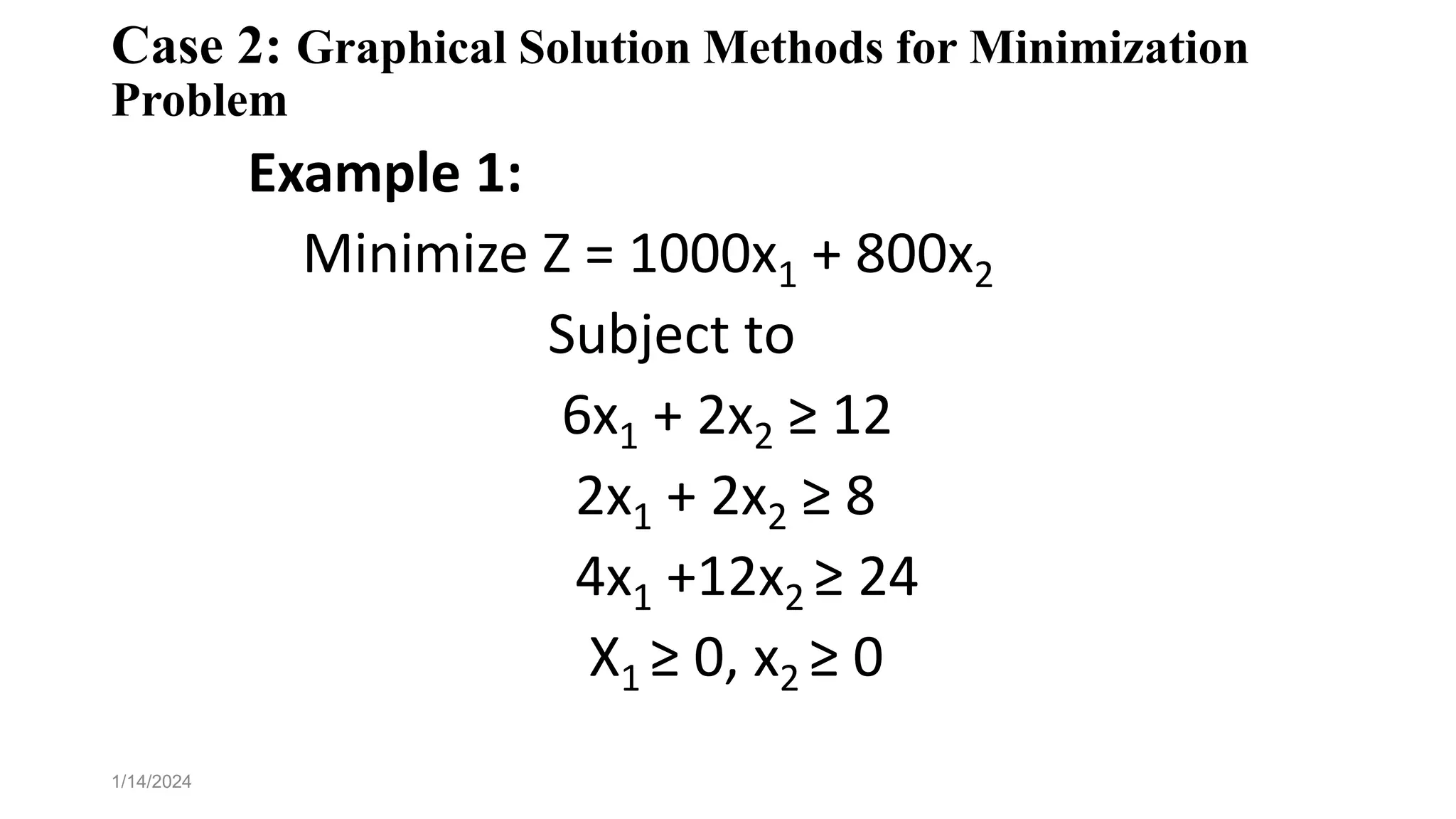
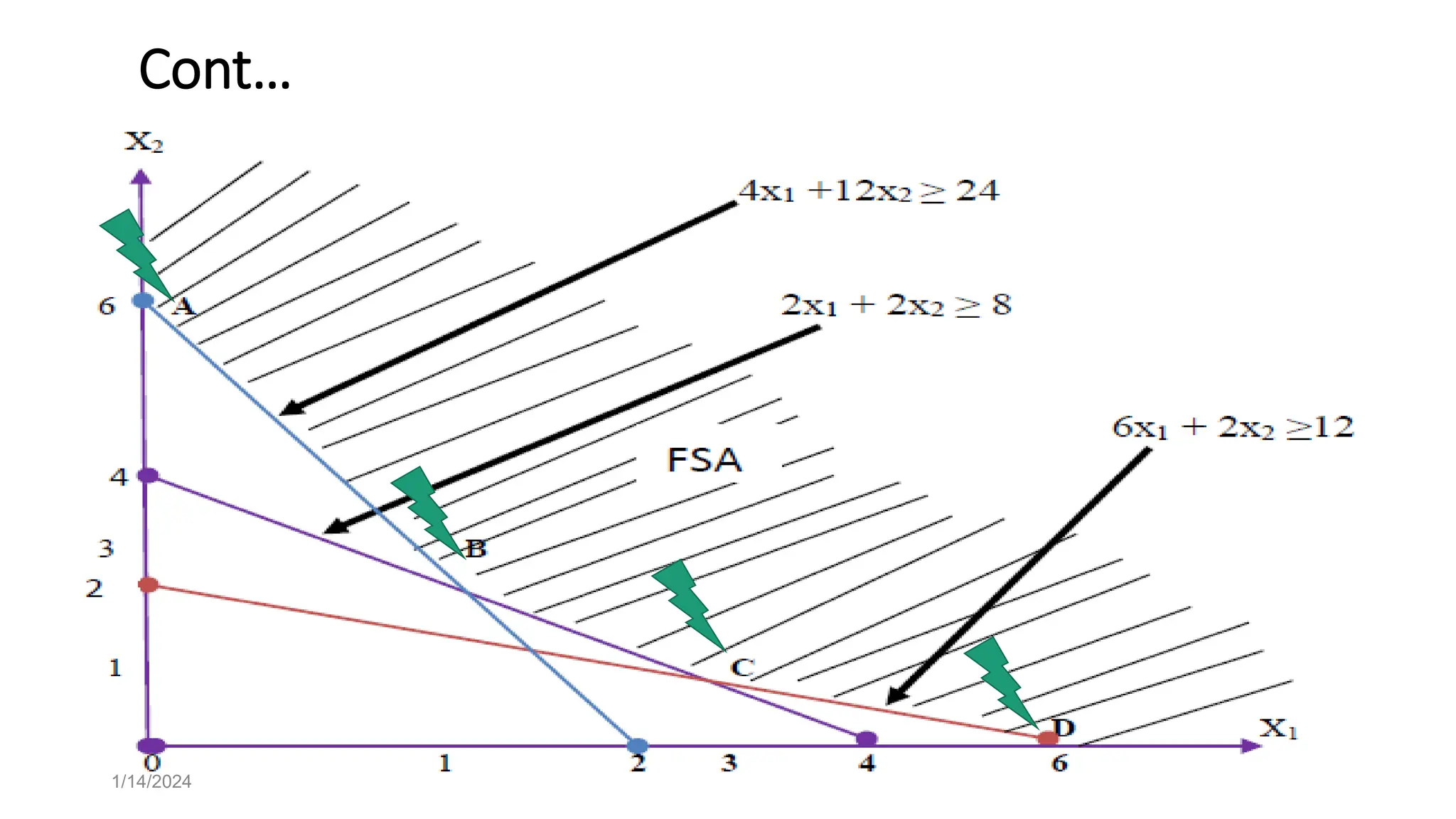
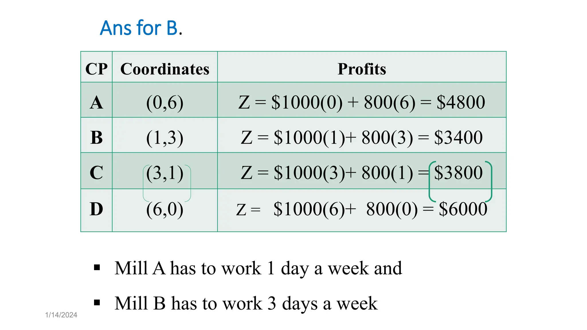
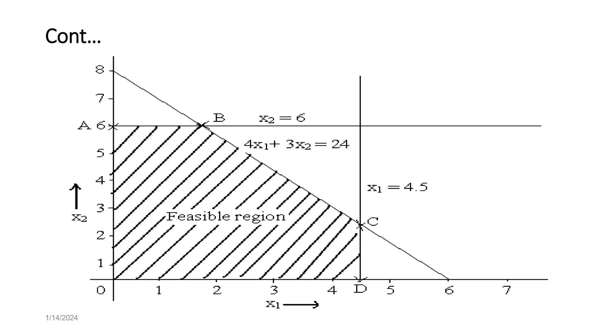
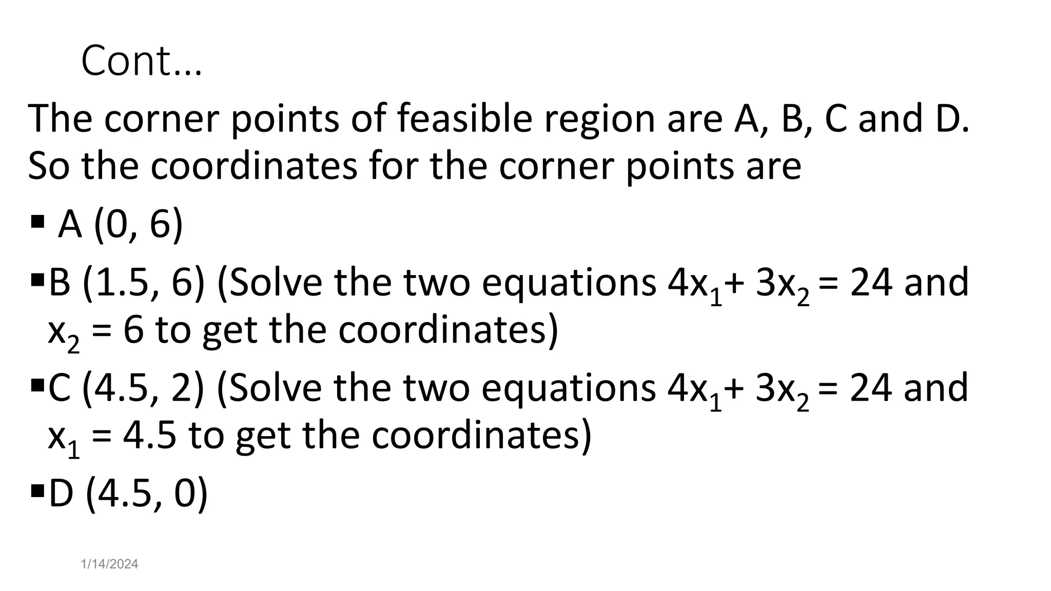
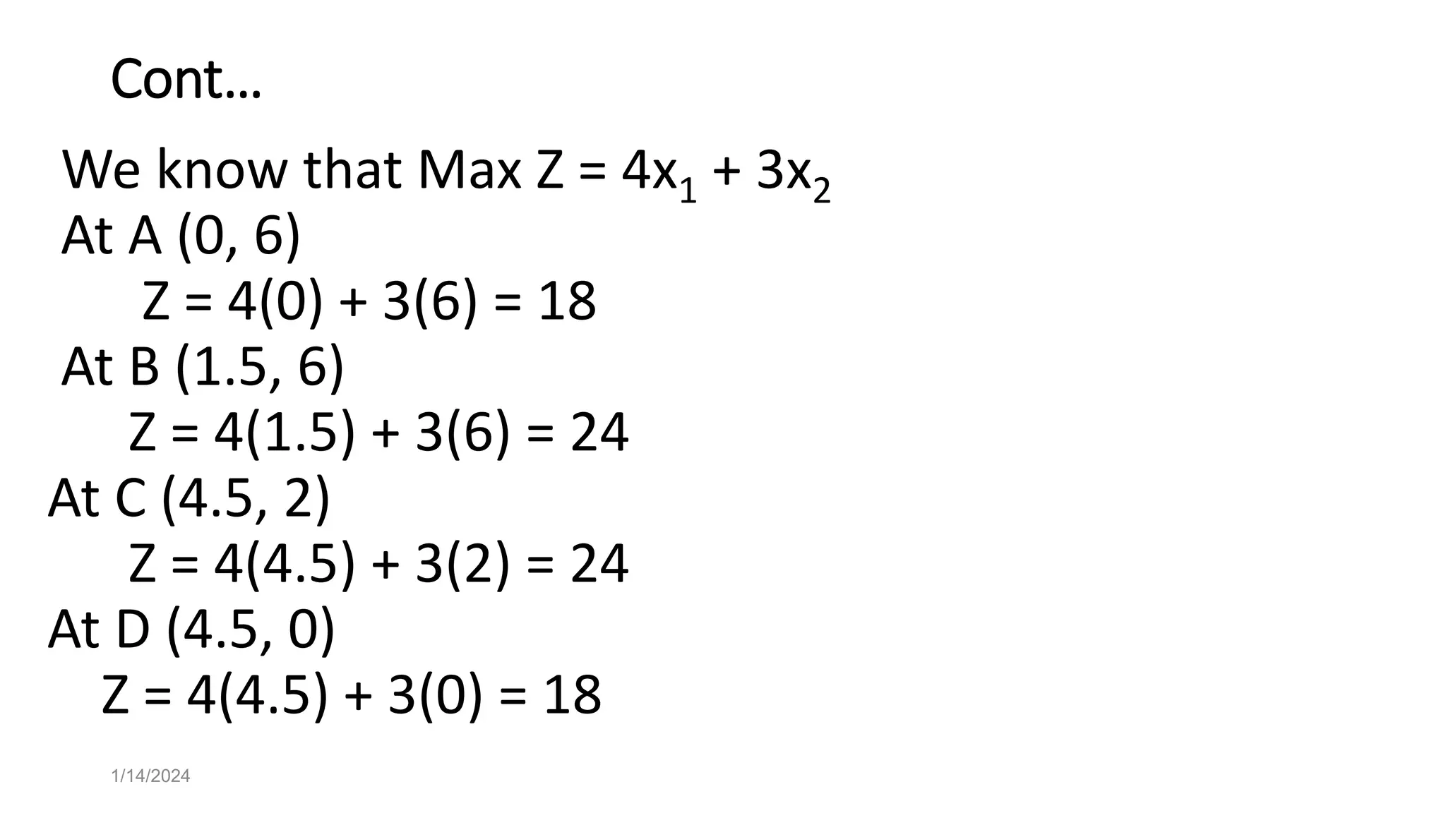
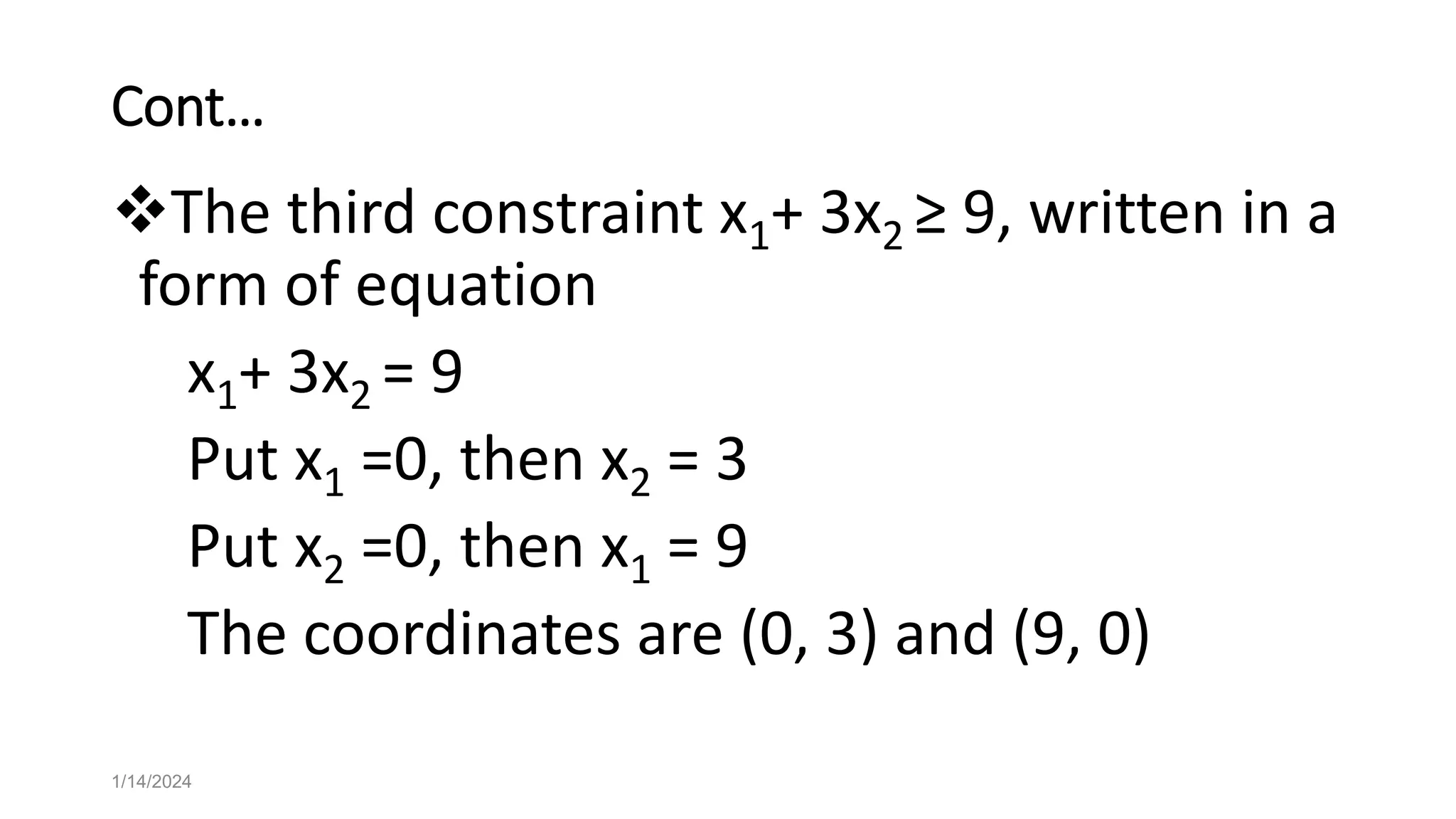
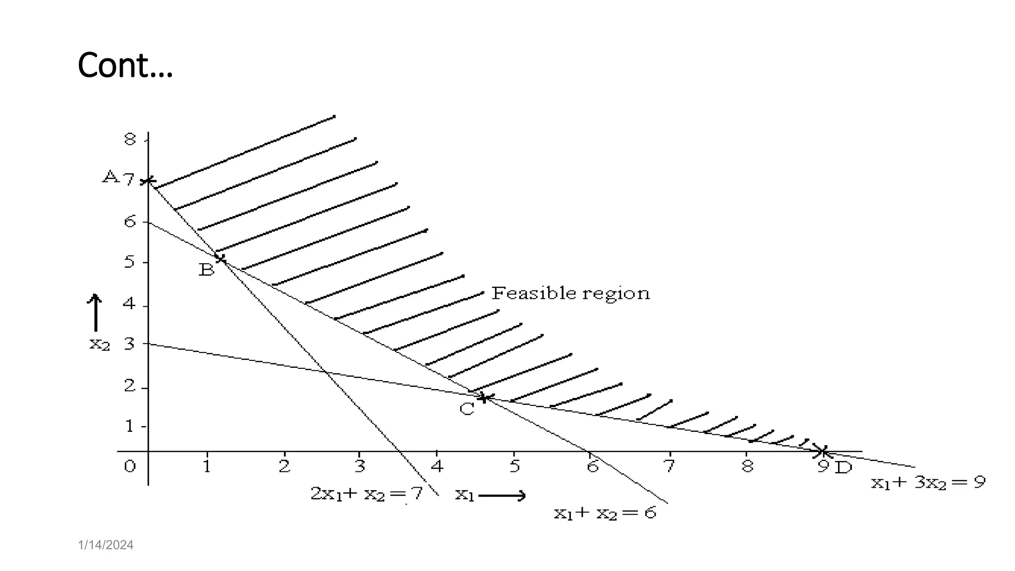
Mathematics For Management CHAPTER THREE PART I.PPT
1. CHAPTER THREE
LINEAR PROGRAMMING
Definition:
Linear programming is a technique applied for
the optimizing a linear objective function, subject to linear
equality and linear inequality constraints.
Is a particular technique used for economic allocation of
‘scarce’ or ‘limited’ resources.
1/14/2024
2. Cont…
e.g. labour, material, machine, time,
warehouse space, capital, energy, etc.:
several competing activities e.g. products,
services, jobs, new equipment, projects, etc. on
the basis of a given criterion of optimality.
1/14/2024
3. Components of LPP
The linear programming model consists of the
following components:
Decision variables: mathematical symbols representing levels
of activity of an operation.
Objective function: a linear relationship reflecting the objective
of an operation.
Constraint: a linear relationship representing a restriction on
decision making.
Non-negativity: values of the decision variables are zero or
non-zero positives.
1/14/2024
4. General form of LP
Z = c1x1 + c2x2 +…………. +cnxn
Subject to restrictions
a11x1 + a12x2 + …..........+a1nxn (≤ or ≥) b1
a21x1 + a22x2 + …………..+a2nxn (≤ or ≥) b2
.
am1x1 + am2x2 + ………. +amnxn (≤ or ≥) bm &
x1 ≥ 0, x2 ≥ 0,…, xn ≥ 0
1/14/2024
5. Cont…
Where
Z = value of overall measures of performance
xj = level of activity (for j = 1, 2, ...,n)
cj = a unit profit/cost increase in Z that would result from
each unit increase in the decision variables (j=1,2, . . .,n)
bi = amount of resource i that is available for allocation to
each decision variables (for i = 1,2, …, m)
aij = amount of resource i consumed by each unit of activity j
1/14/2024
6. Cont. . .
Resource
Resource usage per unit of activity Amount of
resource
available
Activity
1 2 …………………….. n
1
2
.
.
.
M
a11 a12 …………………….a1n
a21 a22 …………………….a2n
.
.
.
am1 am2 …………………amn
b1
b2
.
.
.
Bm
Contribution to Z per
unit of activity
C1, c2 ……………………….cn
1/14/2024
7. Linear Programming Model Construction
General steps taken are as under:
Define the decision variables .
Identify the coefficient of each decision variables.
Formulate the objective function.
Identify the coefficients of each decision variables in the obj fun.
Identify the constrained resources or RHS values.
Formulate the suitable mathematical constraints related to each
respective resource.
Mention the non-negativity constraints associated with the
decision variables.
1/14/2024
8. Assumptions of Linear Programming
Proportionality
Additive
Divisibility
Deterministic
Finiteness
Optimality
One objective
1/14/2024
9. Profit Maximization case
Example 1: Problem Definition
1. A company manufactures two products, tables and chairs by
using three machines A, B, and C so as to maximize a profit.
Machine A has 10 hrs of capacity available during the coming
week. Similarly, the available capacity of machine B and C
during the coming week is 36 hrs and 30 hrs, respectively. One
unit of a table requires 2 hrs of machine A, 3 hrs of machine B
and 3 hrs of machine C. Similarly, one unit of a chair requires 1
hr, 12 hrs and 6 hrs of machine A, B, and C respectively. When
one unit of table is produced and sold, it yields a profit of Birr
5 and that of a chair is Birr 7. Given the above information,
formulate the linear programming model.
1/14/2024
10. Solution
I. Decision variable
how tables and chairs can the managers produce?
the quantities to be produced can be denoted as:
X1: number of tables to be produced
X2: number of chairs to be produced
II. The Objective function
It is to max profit (sum of each)
Then total profit = $5x1+ 7x2 i.e.
1/14/2024
11. Cont…
III. Model Constraints
three resources are used for production are hours of
machine A, B, and C respectively.
hours of machine A constraint is 2x1+ 1x2 ≤ 10
hours of machine B constraint is 3x1 + 12x2 ≤36
hours of machine C constraint is 3x1 + 6x2 ≤ 30
IV. Non-negativity constraint:
x1 ≥ 0, x2 ≥ 0.
1/14/2024
12. Cont. . .
The complete linear programming model for
this problem can now be summarized
bellow as
Max Z = $5x1+ 7x2
ST: 2x1 + 1x2 ≤ 10
5x1 + 2x2 ≤ 36
3x1 + 6x2 ≤ 30
x1, x2 ≥ 0
1/14/2024
13. Example 2: Problem Definition
• Example1: Assume ‘XY’ company is a small craft operation run by a
Native American tribal council. The company employs skilled artisans
to produce clay bowls and mugs with authentic Native American
designs and colours. The company also employed inspectors who will
check the products after finished. The three primary resources used
by the company are special pottery clay, skilled labour and inspectors.
Given these limited resources, the company desires to know how
many bowls and mugs to produce each day in order to max profit.
The two products have the following resource requirements for
production and profit per item produced (i.e. the model parameters).
1/14/2024
14. Example 1: Problem Definition . . .
Resource requirement
Product Labor Inspector Clay Profit
Hr/unit Hr/Unit Ib/unit $/unit
Bowl 2 1 5 50
Mug 2 4 2 35
There are 40 hours of labour 50 hours of inspector and 60 pounds of
clay available each day for production.
Required: Formulate the LP model of this problem.
1/14/2024
15. Example 1: Problem Definition . . .
The final complete LP model
Max Z = $50x1 + 35x2
ST: 2x1 + 2x2 ≤ 40
5x1 + 2x2 ≤ 50
x1 + 4x2 ≤ 60
x1, x2 ≥ 0
1/14/2024
16. Exercise 1
A firm manufactures two types of products A and B and sells them at a profit of
$2 on type A and $3 on type B. Each product is processed on two machines G
and H. Type A requires 1 minute of processing time on G and 2 minutes on H;
type B requires 1 minute on G and 1 minute on H. The machine G is available for
not more than 6 hours 40 minutes while machine H is available for 10 hours
during any working day.
Required: a) Formulate the problem as a linear programming problem
b) Solve the problem using graphical method
Answer for que a)
Maximize Z = 2x1 + 3x2
ST X1 + x2 ≤ 400
2x1 + 3x2 ≤ 600
X1 ≥ 0, x2 ≥ 0
17. Cost Minimization case – Example 1
A company owns 2 oil mills A and B which have
different production capacities for low, high and
medium grade oil. The company enters into a
contract to supply oil to a firm every week with 12, 8,
24 barrels of each grade respectively. It costs the
company $1000 and $800 per day to run the mills A
and B. On a day A produces 6, 2, 4 barrels of each
grade and B produces 2, 2, 12 barrels of each grade.
Required: Develop the LP model.
1/14/2024
18. Solution
Let x1 be the number of days a week the mill A has to work
x2 be the number of days per week the mill B has to work
1/14/2024
Grade A B Minimum requirement
Low 6 2 12
High 2 2 8
Medium 4 12 24
Cost per day $1000 $800
19. Cont…
Therefore, the complete LP model is;
Minimize Z = 1000x1 + 800 x2
Subject to
6x1 + 2x2 ≥ 12
2x1 + 2x2 ≥ 8
4x1+12x2 ≥ 24
x1 ≥ 0, x2 ≥ 0
1/14/2024
20. Optimal Solution Methods
There are two approaches to solve linear
programming problems:
The Graphical Algorithm
The Simplex Algorithm
1/14/2024
21. Graphical Method
A graphical approach is limited to linear
programming problems with only two decision
variables.
The complexity of its application increases as
the number of constraint functions increases.
It is a relatively straightforward method for
determining the optimal solution to certain linear
programming problems.
1/14/2024
22. The following are the steps to be followed in solving LP
problems graphically:
Formulate the problem in terms of mathematical
constraints and an objective function.
Convert the inequalities into equation and compute the
coordinate points
Plot the model constraints on the graph
Identify the feasible region i.e. the area which satisfies all
the constraints simultaneously
1/14/2024
23. Cont…
Plot the objective function then move the line out from the
origin till it touches the extreme maximum points of the
feasible solution area.
Plot the objective function then move the line down till it
touches the extreme minimum point of the feasible solution
area.
Substitute these values into the objective function to find the
set of values that result in the maximum profit or the
minimum cost.
Interpreting the results
1/14/2024
24. Cont. . .
Case 1: Graphical Solution Method for Maximization Problem
Example 1: Max Z = $50x1+ 35x2
ST: 2x1 + 2x2 ≤ 40
5x1 + 2x2 ≤ 50
x1 + 4x2 ≤ 60
x1, x2 ≥ 0
Required: Compute the optimal solution using graphical
method. Apply all possible steps.
1/14/2024
25. Solution:
First develop the problem into mathematical linear
programing if not given.
The structured model is given so we need to proceed
into change the inequalities into equations for
computing the coordinate points.
2x1 + 2x2 = 40
5x1 + 2x2 = 50
x1 + 4x2 = 60
1/14/2024
28. Cont…
In this graph, the FSA is represented by the shaded
region.
The feasible region has four corner points i.e. O, A, B,
and C.
From these corner points at least one will give us
maximum profit
The one that generate the highest profit would be
regarded as optimal corner point/s.
1/14/2024
33. Cont…
Interpretation
Form this result; we can conclude that the
manager has different alternatives to make
decisions but since the objective of the
problem is to maximize profit, she has to
select the best alternative i.e. alternative
corner point B at x1 = 40/9 and x2 = 125/9
1/14/2024
34. Case 2: Graphical Solution Methods for Minimization
Problem
Example 1:
Minimize Z = 1000x1 + 800x2
Subject to
6x1 + 2x2 ≥ 12
2x1 + 2x2 ≥ 8
4x1 +12x2 ≥ 24
X1 ≥ 0, x2 ≥ 0
1/14/2024
35. Cont…
Required:
A. Sketch the graph and identify the feasible solution
area
B. How many numbers of products type x1 and type x2
the company has to produce to minimize cost?
C. What is the z value of the problem?
D.Does the problem have unique solution? Why?
1/14/2024
36. Ans for A.
To sketch the graph, determine the CPs of each constraint by
changing the ≥ into =
6x1 + 2x2 = 12
Let x1 = 0, x2 = 6 coordinate points = (0, 6)
Let x2 = 0, x1 = 2 coordinate points = (2, 0)
2x1 + 2x2 = 8
Let x1 = 0, x2 = 4 coordinate points = (0, 4)
Let x2 = 0, x1 = 4 coordinate points = (4, 0)
4x1 +12x2 = 24
• Let x1 = 0, x2 = 2 coordinate points = (0, 2)
•Let x2 = 0, x1 = 6 coordinate points = (6, 0)
1/14/2024
38. Ans for B.
CP Coordinates Profits
A (0,6) Z = $1000(0) + 800(6) = $4800
B (1,3) Z = $1000(1)+ 800(3) = $3400
C (3,1) Z = $1000(3)+ 800(1) = $3800
D (6,0) Z = $1000(6)+ 800(0) = $6000
1/14/2024
Mill A has to work 1 day a week and
Mill B has to work 3 days a week
39. Ans for C.
The optimal solution or the minimum possible cost of
the problem is $3400.
Ans for D
The answer is yes because the company has no
alternatives days to work more or less for both mill A
and mill B without changing the minimum possible
cost.
1/14/2024
40. Graphical Solution of Irregular Types of Linear
Programming Problems:
If a linear programming problem has a unique
solution, then it must occur at a corner point of the
feasible set.
However, there are several special types of typical
linear programming problems (linear programming
models for which the general rules do not always
apply).
1/14/2024
41. These special types of linear programming problems
include the following:
A. Multiple optimal solutions
B. Infeasible problem
C. Unbounded problem
D. Redundancy
1/14/2024
42. A. Multiple optimal solutions
If the objective function is optimized at two adjacent
corner points of the feasible area, it is optimized at
every point on the line segment joining these corner
points, in which case there are infinitely many solutions
to the problem.
Multiple optimal solutions can benefit the decision
maker since the number of decision options is enlarged.
Multiple optimal solutions provide greater flexibility
to the decision maker.
1/14/2024
43. Con…
Example 1:
Max Z = 4x1 + 3x2
Subject to
4x1+ 3x2 ≤ 24
x1 ≤ 4.5
x2 ≤ 6
x1 ≥ 0, x2 ≥ 0
1/14/2024
44. Solution
The first constraint 4x1+ 3x2 ≤ 24, written in a form of
equation
4x1+ 3x2 = 24
Put x1 =0, then x2 = 8
Put x2 =0, then x1 = 6
The coordinates are (0, 8) and (6, 0)
1/14/2024
45. Cont…
The second constraint x1 ≤ 4.5, written in a form of
equation
x1 = 4.5
The third constraint x2 ≤ 6, written in a form of
equation
x2 = 6
1/14/2024
47. Cont…
The corner points of feasible region are A, B, C and D.
So the coordinates for the corner points are
A (0, 6)
B (1.5, 6) (Solve the two equations 4x1+ 3x2 = 24 and
x2 = 6 to get the coordinates)
C (4.5, 2) (Solve the two equations 4x1+ 3x2 = 24 and
x1 = 4.5 to get the coordinates)
D (4.5, 0)
1/14/2024
48. Cont…
We know that Max Z = 4x1 + 3x2
At A (0, 6)
Z = 4(0) + 3(6) = 18
At B (1.5, 6)
Z = 4(1.5) + 3(6) = 24
At C (4.5, 2)
Z = 4(4.5) + 3(2) = 24
At D (4.5, 0)
Z = 4(4.5) + 3(0) = 18
1/14/2024
49. Cont…
Max Z = 24, which is achieved at both B and C
corner points. It can be achieved not only at
B and C but every point between B and C.
Hence the given problem has multiple
optimal solutions.
1/14/2024
50. B. No Optimal Solution/infeasible solution
An infeasible solution has no feasible solution
area; every possible solution point violates one
or more constraints. In other words, if a
solution violates at least one constraint, the
solution is said to be infeasible.
1/14/2024
52. Cont…
Solution
The first constraint x1+ x2 ≤ 1 is written in the
form of x1+ x2 = 1
Put x1 =0, then x2 = 1
Put x2 =0, then x1 = 1
The coordinates are (0, 1) and (1, 0)
1/14/2024
53. Cont…
The second constraint x1+ x2 ≥ 3, written in a form of
equation
x1+ x2 = 3
Put x1 =0, then x2 = 3
Put x2 =0, then x1 = 3
The coordinates are (0, 3) and (3, 0)
1/14/2024
55. Cont…
There is no common feasible region generated by
two constraints together i.e. we cannot identify
even a single point satisfying the constraints.
Hence there is no optimal solution.
1/14/2024
56. C. Unbounded Solution
In an unbounded problem, the feasible solution area
formed by the model constraints is not closed.
In unbounded problem the objective function can
increase indefinitely without reaching a maximum
value.
Unlimited profits are not possible in the real world;
and an unbounded solution, like an infeasible
solution, typically reflects an error in defining the
problem or in formulating the model.
1/14/2024
57. Cont…
Example1: Solve by graphical method
Max Z = 3x1 + 5x2
Subject to
2x1+ x2 ≥ 7
x1+ x2 ≥ 6
x1+ 3x2 ≥ 9
x1 ≥ 0 , x2 ≥ 0
1/14/2024
58. Cont…
Solution
The first constraint 2x1+ x2 ≥ 7, written in a
form of equation
2x1+ x2 = 7
Put x1 =0, then x2 = 7
Put x2 =0, then x1 = 3.5
The coordinates are (0, 7) and (3.5, 0)
1/14/2024
59. Cont…
The second constraint x1+ x2 ≥ 6, written in a
form of equation
x1+ x2 = 6
Put x1 =0, then x2 = 6
Put x2 =0, then x1 = 6
The coordinates are (0, 6) and (6, 0)
1/14/2024
60. Cont…
The third constraint x1+ 3x2 ≥ 9, written in a
form of equation
x1+ 3x2 = 9
Put x1 =0, then x2 = 3
Put x2 =0, then x1 = 9
The coordinates are (0, 3) and (9, 0)
1/14/2024
62. Cont…
The corner points of feasible region are A, B, C and D. So the
coordinates for the corner points are:
A (0, 7)
B (1, 5) (Solve the two equations 2x1+ x2 = 7 and x1+ x2 = 6
to get the coordinates)
C (4.5, 1.5) (Solve the two equations x1+ x2 = 6 and x1+ 3x2 =
9 to get the coordinates)
D (9, 0)
1/14/2024
63. D. Redundancy
A redundant constraint is simply one that does not
affect the feasible solution region.
One constraint may be more binding or restrictive than
the other and thereby negate its need to be considered.
1/14/2024