
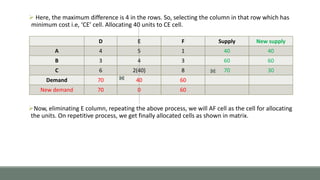
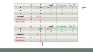
![Since, the matrix is balanced; we should start from step 2.
Here, finding out the difference between the smallest and second smallest for each row and
each column & entering in respective column and row. It is shown in brackets.
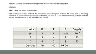
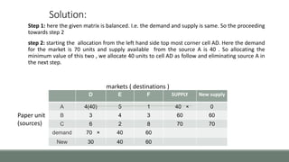
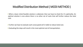
Example :- The paper manufacturing company has three warehouses located in
three different areas, says A, B & C. The company has to send from these
warehouses to three destinations, says D, E & F. The availability from warehouses A,
B & C is 40, 60, & 70 units. The demand at D, E and F is 70, 40 and 60 respectively.
The transportation cost is shown in matrix (in Rs.).
D E F Supply Row Difference
A 4 5 1 40 [3]
B 3 4 3 60 [0]
C 6 2 8 70 [4]
Demand 70 40 60 170
Column Difference [1] [2] [2]](https://image.slidesharecdn.com/orpptnew-160716061403/85/MODI-Method-Operations-Research-9-320.jpg)
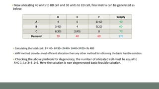
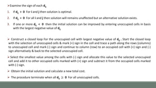
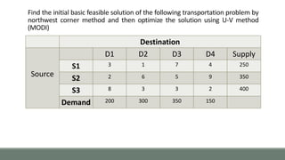
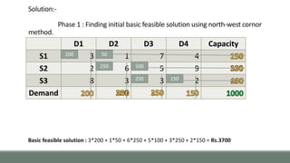
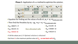

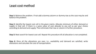
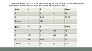
The document outlines the presentation topic of Modified Distribution Method (MODI Method) for solving transportation problems. It first discusses the prerequisite methods of Least Cost Method, Vogel's Approximation Method and North-West Corner Method. It then explains the steps of MODI Method which involves setting up cost matrices for unallocated cells and introducing dual variables to find the implicit cost and evaluate unoccupied cells to determine if the initial solution can be improved. The document provides an example problem and solution to demonstrate the application of MODI Method.