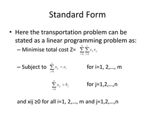
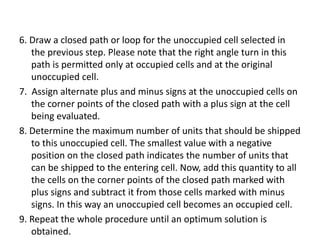
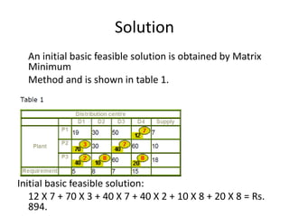
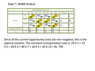
The document describes the modified distribution method (MODI) for solving transportation problems. MODI is an improvement on the stepping stone method. It involves starting with an initial basic feasible solution, calculating opportunity costs, and finding a negative opportunity cost to enter a new cell into the solution. A closed path is drawn around this cell and units are added/subtracted along the path to create a new basic feasible solution. This process repeats until all opportunity costs are non-negative, indicating an optimal solution. An example demonstrates applying MODI to find the optimal solution that minimizes transportation costs.

1. Modified Distribution Method
Prepared by:
Mayank N. Lathewala 130110119048
Mharshi H. Soni 130010119050
Mahmadfaizal I. Ghanchivohra 130010119052
Submitted to: Dr. Unnati A. Joshi
Subject of : Operations Research

2. Introduction
• The transportation problem and cycle canceling
methods are classical in optimization.
• The transportation problem is concerned with finding
an optimal distribution plan for a single commodity.
• A given supply of the commodity is available at a
number of sources, there is a specified demand for the
commodity at each of a number of destinations, and
the transportation cost between each source-
destination pair is known.
• In the simplest case, the unit transportation cost is
constant.
• The problem is to find the optimal distribution plan for
transporting the products from sources to destinations
that minimizes the total transportation cost.

3. Here sources indicated the place from where transportation will begin,
destinations indicates the place where the product has to be arrived
and cij indicated the transportation cost transporting from source to
destination and Sink denotes the destination.

4. Unbalanced Transportation Problem
• A Transportation Problem is said to be unbalanced
transportation problem if total number of supply is not
same as total number of demand.
• TP can also be formulated as linear programming
problem that can be solved using either dual simplex or
Big M method and also by using interior approach
method.
• Vogel’s method gives approximate solution while MODI
and Stepping Stone (SS) method are considered as a
standard technique for obtaining to optimal solution.

5. Mathematical Statement of the
Problem
• The classical transportation problem can be
stated mathematically as follows:
– Let ai denotes quantity of product available at
origin i, bj denotes quantity of product required at
destination j, Cij denotes the cost of transporting
one unit of product from source/origin i to
destination j and xij denotes the quantity
transported from origin i to destination j.

6. Assumptions:
• This means that the total quantity available at the
origins is precisely equal to the
• total amount required at the destinations. This
type of problem is known as
• balanced transportation problem. When they are
not equal, the problem is called
• unbalanced transportation problem. Unbalanced
transportation problems are
• then converted into balanced transportation
problem using the dummy variables.

7. Standard Form
• Here the transportation problem can be
stated as a linear programming problem as:
– Minimise total cost Z=
– Subject to for i=1, 2,…, m
for j=1,2,…,n
and xij ≥0 for all i=1, 2,…, m and j=1,2,…,n

8. The transportation model can also be portrayed in a tabular
form by means of a transportation table, shown in Table 3.1.

9. MODI
• The modified distribution method, MODI for
short , is an improvement over the stepping
stone method for testing and finding optimal
solutions.

10. Steps
1. Determine an initial basic feasible solution using any one of the
three given methods which are namely, North West Corner
Method, Least Cost Method and Vogel Approximation Method.
2. Determine the values of dual variables, ui and vj, using ui + vj =
cij
3. Compute the opportunity cost using dij= cij – (ui + vj) from
unoccupied cell.
4. Check the sign of each opportunity cost (dij). If the opportunity
costs of all the unoccupied cells are either positive or zero, the
given solution is the optimum solution. On the other hand, if
one or more unoccupied cell has negative opportunity cost, the
given solution is not an optimum solution and further savings in
transportation cost are possible.
5. Select the unoccupied cell with the smallest negative
opportunity cost as the cell to be included in the next solution.

11. 6. Draw a closed path or loop for the unoccupied cell selected in
the previous step. Please note that the right angle turn in this
path is permitted only at occupied cells and at the original
unoccupied cell.
7. Assign alternate plus and minus signs at the unoccupied cells on
the corner points of the closed path with a plus sign at the cell
being evaluated.
8. Determine the maximum number of units that should be shipped
to this unoccupied cell. The smallest value with a negative
position on the closed path indicates the number of units that
can be shipped to the entering cell. Now, add this quantity to all
the cells on the corner points of the closed path marked with
plus signs and subtract it from those cells marked with minus
signs. In this way an unoccupied cell becomes an occupied cell.
9. Repeat the whole procedure until an optimum solution is
obtained.

12. Example
Total Cost: 3*20 + 4*15 + 8*20 +4*60 + 1*35 = Rs. 555
This routing of the units meets all the rim requirements and
entails 5 (=m+n-1 = 3+3-1) shipments as there are 5 occupied
cells; It involves a total cost of Rs. 555.

13. Example
• Consider the transportation problem
presented in the following table.
Determine the optimal solution of the above
problem.

14. Solution
An initial basic feasible solution is obtained by Matrix
Minimum
Method and is shown in table 1.
Initial basic feasible solution:
12 X 7 + 70 X 3 + 40 X 7 + 40 X 2 + 10 X 8 + 20 X 8 = Rs.
894.

16. Now choose the smallest (most) negative value from
opportunity cost (i.e., –13) and draw a closed path
from P1D1. The following table shows the closed
path.

17. • Choose the smallest value with a negative position on the closed
path(i.e., 2), it indicates the number of units that can be shipped
to the entering cell. Now add this quantity to all the cells on the
corner points of the closed path marked with plus signs and
subtract it from those cells marked with minus signs. In this way,
an unoccupied cell becomes an occupied cell.

18. Now again calculate the values for ui & vj and opportunity cost.
The resulting matrix is shown below.
Now choose the smallest (most) negative value from
opportunity cost (i.e., –13) and draw a closed path
from P1D1. The following table shows the closed path.

19. Now again calculate the values for ui & vj and
opportunity cost.

20. Since all the current opportunity costs are non–negative, this is the
optimal solution. The minimum transportation cost is: 19 X 5 + 12
X 2 + 30 X 3 + 40 X 7 + 10 X 5 + 20 X 13 = Rs. 799