Lecture 9&10 computer vision segmentation-no_task

Computer Vision
SBE 404, Spring 2020
Professor
Ahmed M. Badawi
ambadawi@eng1.cu.edu.eg
http://scholar.google.com.eg/citations?user=r9pLu6EAAAAJ&hl=en
http://www.bmes.cufe.edu.eg
TA’s:
Eman Marzban
eman.marzban@eng1.cu.edu.eg
Asem Abdelaziz
asem.a.abdelaziz@eng1.cu.edu.eg

Segmentation
Images objects
How?
Similarity, homogeneity
− The goal of segmentation is to partition an image into regions (e.g.,
separate objects from background) sharing similar properties.
− Segmentation is sometimes very difficult problem in general !!

It is difficult. How to increase
accuracy and robustness?
− Introduce enough knowledge about the application domain (Model
or Atlas, parametric vs non-parametric)
− Assume control over the environment (e.g., in industrial
applications)
− Select type of sensors to enhance the objects of interest (e.g., use
infrared imaging for target recognition applications)
Readings: Szeliski Chapter 5.
Recommended readings Forsyth & Ponce, Chapter 7.
Milan Sonka, Chapter 6.

Segmentation is a classification
(clustering) problem
• Thresholding from histogram modes(eg. Optimal
thresholding and Otsu). Bimodal and spectral
• Edge based (eg. Hough transform, snake, graph
cuts, graph search, link cost function, and
shortest path for scissors)
• Region based (merging and splitting or region
growing)
• Matching (finding object or template in image)
• Evaluation (supervised vs unsupervised), ROC

Thresholding
• The simplest approach to image segmentation is by
thresholding:
if f(x,y) < T then f(x,y) = 0 else f(x,y) = 255
Some slides are from Steve Seitz (R. Szeliski book), James Hayes, Sonka, and Shapiro
book.

Finding thresholds
There are many methods to
automatically find the optimum (in
some sense) threshold from a
histrogram,
Note that there will often be
misclassified pixels, they have to be
handled when forming the regions.
Histogram based (no spatial
or neighborhood
dependency)

Thresholding
• Automatic thresholding
− To make segmentation more robust, the threshold should be
automatically selected by the system.
− Knowledge about the objects, the application, the environment
should be used to choose the threshold automatically:
− Intensity characteristics of the objects
− Sizes of the objects
− Fractions of an image occupied by the objects
− Number of different types of objects appearing in an image

Thresholding
• Choosing the threshold using the image histogram
− Problem: some pixels from the
background may look the same as
some pixels from the object
− Solution: hysteresis thresholding

Thresholding
• Hysteresis thresholding
− Two thresholds can be used in this case
− Pixels below the high threshold are classified as object and above
the high threshold as background.
− Pixels between the low and high thresholds are classified as object
only if they are adjacent to other object pixels.
1. if f(x,y) < T1 then f(x,y) = 0 // object
else if T1 < f(x,y) < T2 then f(x,y) = 128 // not sure
else f(x,y) = 255 // background
2. for each (x,y) where f(x,y) = 128
if (x,y) has neighbors (x’,y’) where f(x’,y’) = 0 //object neighbor
f(x,y) = 0 // reassign to object
3. repeat step 2 until no pixels are reassigned
4. for each (x,y) where f(x,y) = 128 // remaining undecided
f(x,y) = 255 // reassign to background

Thresholding
• Hysteresis thresholding

Thresholding
• Using prior knowledge: the P-Tile method
− This method requires knowledge about the area or size of the
objects present in the image
− Assume that there are dark objects against a light background.
− If, for example, the objects occupy p% of the image area, an
appropriate threshold can be chosen by partitioning the histogram

Histogram-based segmentation
• Goal
– Break the image into K regions (segments)
– Solve this by reducing the number of colors to
K and mapping each pixel to the closest color
Slide by S. Seitz

• Goal
Here’s what it looks like if we use two colors
Slide by S. Seitz

Where is optimal threshold
Milan Sonka book chapter 6.

Finding Modes in a Histogram
• How Many Modes Are There?
– Easy to see, hard to compute

Mean Shift [Comaniciu & Meer]
• Iterative Mode Search
1. Initialize random seed, and window W
2. Calculate center of gravity (the “mean”) of W:
3. Translate the search window to the mean
4. Repeat Step 2 until convergence

Thresholding
• Multispectral thresholding
Milan Sonka book chapter 6.

Thresholding
• Otsu’s method (Bimodal distribution)
• A measure of region homogeneity is variance (i.e., regions with high
homogeneity will have low variance).
• Otsu’s method selects the threshold by minimizing the within-class
variance of the two groups of pixels separated by the thresholding
operator.
• It does not depend on modeling the probability density functions,
however, it assumes a bimodal distribution of gray-level values (i.e., if
the image approximately fits this constraint).
• Since the total variance σ does not depend on T, the T minimizing σW
2
will be the T maximizing variance between-class σB
2
• Start from the beginning of the histogram and test each gray-level value
for the possibility of being the threshold T that maximizes σB
2
http://en.wikipedia.org/wiki/Otsu's_method

Otsu’s Thresholding Method
• Based on a very simple idea: Find the
threshold that minimizes the weighted
within-class variance.
• This turns out to be the same as maximizing
the between-class variance.
• Operates directly on the gray level
histogram [e.g. 256 numbers, P(i)], so it’s
fast (once the histogram is computed).
(1979)

Otsu: Assumptions
• Histogram (and the image) are bimodal.
• No use of spatial coherence, nor any other
notion of object structure.
• Assumes stationary statistics, but can be
modified to be locally adaptive. (exercises)
• Assumes uniform illumination (implicitly), so
the bimodal brightness behavior arises from
object appearance differences only.

At specific threshold t, The weighted within-class variance is:
w
2
(t)  q1(t)1
2
(t)  q2 (t)2
2
(t)
Where the class probabilities are estimated as:
q1(t)  P(i)
i1
t
 q2 (t)  P(i)
i t1
I

1(t) 
iP(i)
q1(t)i1
t
 2(t) 
iP(i)
q2(t)it 1
I

And the class means are given by:

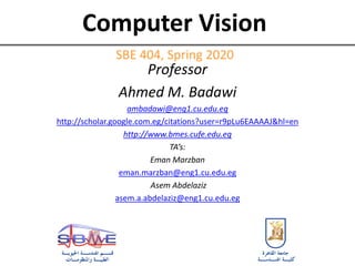
Finally, the individual class variances are:
1
2
(t)  [i  1(t)]
2 P(i)
q1(t)i1
t

2
2
(t)  [i  2(t)]
2 P(i)
q2 (t)it1
I

Now, we could actually stop here. All we need to do is just run through the full
range of t values [1,256] and pick the value that minimizes .
But the relationship between the within-class and between-class
variances can be exploited to generate a recursion relation that permits a much
faster calculation.
w
2
(t) B
2
(t)

Between/Within/Total Variance
• The basic idea is that the total variance does
not depend on threshold (obviously).
• For any given threshold, the total variance is
the sum of the within-class variances
(weighted) and the between class variance,
which is the sum of weighted squared
distances between the class means and the
grand mean.

After some algebra, we can express the total variance as...
2
 w
2
(t) q1(t)[1 q1 (t)][1(t) 2 (t)]
2
Within-class,
from before Between-class,
Since the total is constant and independent of t, the effect of changing the
threshold is merely to move the contributions of the two terms back and forth.
So, minimizing the within-class variance is the same as maximizing the between-
class variance.
The nice thing about this is that we can compute the quantities in
recursively as we run through the range of t values.
B
2
(t)

Finally...
q1(t 1) q1(t) P(t 1)
1(t 1) 
q1(t)1 (t)  (t 1)P(t 1)
q1(t 1)
q1(1)  P(1) 1(0)  0;
2(t 1) 
  q1(t 1)1(t 1)
1  q1(t 1)
Initialization...
Recursion...

Thresholding
• Determining the threshold

Thresholding drawbacks
• Drawbacks of Otsu and other global histogram based
methods
− It assumes that the histogram of the image is bimodal (two classes).
− The method breaks down when the two classes are very unequal
(the classes have very different sizes).
− It does not work well with variable illumination.
- No spatial or neighborhood similarity
- Illumination affecting histogram

Thresholding
• Effect of illumination on segmentation
− How does illumination affect the
histogram?

Thresholding
• Handling non-uniform illumination – laboratory solution
− Obtain an image of just the illumination field.
1. Suppose that f(x, y) = i(x, y) r(x, y), where i(x, y) is non-uniform
2. Project the illumination pattern on a surface with uniform
reflectance (e.g., a white surface)
g(x, y) = k i(x, y)
3. Normalize f (x, y):
h(x, y) = f(x, y) / g(x, y) = r(x, y) / k
4. If r(x, y) can be segmented using T, then h(x, y) can be segmented
using T/k

Thresholding
• Handling non-uniform illumination – local thresholding
− A single threshold will not work well when we have uneven
illumination due to shadows or due to the direction of illumination.
− The idea is to partition the image into m x m subimages (Blocks)
and then choose a threshold Tij for each subimage.
− This approach might lead to sub-images having simpler histograms
(e.g., bimodal)
− Non-stationary but windowing it assumes stationarity in this window
range.

Thresholding
• Handling non-uniform illumination – local thresholding

Region Growing
• The fundamental drawback of histogram-based region
detection is that histograms provide no spatial information
(only the distribution of gray levels).
• Region-growing approaches exploit the important fact that
pixels which are close together have similar gray values.
• Region growing
− Start with a single pixel (seed) and add new pixels

Region Growing
• More than one seed
can be used

Region Growing
• How do we choose the seed(s) in practice ?
− It depends on the nature of the problem
− If targets need to be detected using infrared images for example,
choose the brightest pixel(s).
− Without prior knowledge, compute the histogram and choose the
gray-level values corresponding to the strongest peaks (e.g., 1 and
7 in the previous example)

Region Growing
• How do we choose the similarity criteria (predicates)?
− The homogeneity predicate can be based on any characteristic of
the regions in the image, such as:
− average intensity
− variance
− color
− texture
− motion
− shape
− size
• Region growing based on simple surface fitting
• If the errors are small, then we can conclude that the pixel values belong to the
same region.

Region Growing
• Problems
− The main assumption of this approach is that regions are nearly
constant or have smooth variations in image intensity.
− This approach will not work for non-smoothly varying regions (e.g.,
textured regions).
− More sophisticated approaches are required to allow for more
realistic intensity variations due to shading.

Split and merge regions (QuadTrees)
The regions found using the previous methods are uniquely
homogenous, resulting in a Boolean Homogeneous Criteria function H(R)
with:
H( Rk ) = true for all regions k
H( Ri  Rj ) = false for i  j combined regions
For example | f(x,y) - f(x',y')| < T , the regions pass the peak test.
Horowitz and Pavlides (1974) organize the image pixels into a (pyramid) grid structure. Every
region (except for 1 pixel areas) can be split up into 4 regions. Four regions on the correct
position can be joined again to make 1 region.
They used this structure in the following split and merge join algorithm working for every
function H():
- begin with all the regions on a satisfactory level in the pyramid.
- if there is a Rk with H(Rk) = false, then divide the Rk into four even parts.
- if for the 4 sub regions, lying on the correct position, the following holds
H( Rk1  Rk2  Rk3  Rk4) = true, then join the 4 sub regions together to Rk.
- repeat the last two steps until there is nothing left to divide or join
- finally join the regions together that do not fit into the pyramid structure neatly.

Although it is common to start with the single region assumption, it is possible to start at an
intermediate level, e.g. 16 regions or whatever. In the latter case, it is possible that 4 regions may be
merged to form a parent region. For simplicity, assume we start with a single region, i.e. the whole
image. Then, the process of splitting is simple. A list of current regions to be processed, i.e. regions
defined as not homogeneous is maintained. When a region is found to be homogeneous it is
removed from the ProcessList and placed on a RegionList.
Splitting and merging attempts to divide an image into uniform regions. The basic representational
structure is pyramidal, i.e. a square region of size m by m at one level of a pyramid has 4 sub-regions
of size m/2 by m/2 below it in the pyramid. Usually the algorithm starts from the initial assumption
that the entire image is a single region, then computes the homogeneity criterion to see if it is TRUE.
If FALSE, then the square region is split into the four smaller regions. This process is then repeated on
each of the sub-regions until no further splitting is necessary. These small square regions are
then merged if they are similar to give larger irregular regions. The problem (at least from a
programming point of view) is that any two regions may be merged if adjacent and if the larger region
satisfies the homogeneity criteria, but regions which are adjacent in image space may have different
parents or be at different levels (i.e. different in size) in the pyramidal structure. The process
terminates when no further merges are possible.

Best Merge
First all the 4-connected pixels are joined into one region if they are exactly alike.
Then the two 4-connected regions with the smallest error criteria for merging are
combined together to 1 region. This is repeated until the error criteria is larger
than a certain threshold. Choosing the “right” stopping value is a difficut problem.
For the Landsat satellite image, the error criteria between two regions i and j was:
Eij =  (  c ( c
i -  c
j)2
 c
k is the average value of the area k in band c
Also other E’s could be used, e.g. taking the size of the regions to favour merging of
small regions with large ones. Also the ’s of the regions could be taken into
account.

Region growing
Image showing defective welds
Selected “seed” points, pixels
with a value of 255.
Result of region growing according
to certain criteria.
Boundaries of segmented
defective welds.

example Landsat
1 band, threshold 6
1 band, threshold 10
1 band, threshold 16
all bands, threshold 6

Clustering example: image segmentation
Goal: Break up the image into meaningful or
perceptually similar regions
Slides by James Hayes

Segmentation for feature support
50x50 Patch50x50 Patch
Slide: Derek Hoiem

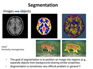
Segmentation for efficiency
[Felzenszwalb and Huttenlocher 2004]
[Hoiem et al. 2005, Mori 2005]
[Shi and Malik 2001]
Slide: Derek Hoiem

Segmentation as a result
Rother et al. 2004

Types of segmentations
Oversegmentation Undersegmentation
Multiple Segmentations

Clustering: group together similar points and
represent them with a single token (Label)
Key Challenges:
1) What makes two points/images/patches similar?
2) How do we compute an overall grouping from
pairwise similarities?
Slide: Derek Hoiem
Clustering means grouping based on similarity

Why do we cluster?
• Summarizing data
– Look at large amounts of data
– Patch-based compression or denoising
– Represent a large continuous vector with the cluster number
• Counting
– Histograms of texture, color, SIFT vectors
• Segmentation
– Separate the image into different regions
• Prediction
– Images in the same cluster may have the same labels
Slide: Derek Hoiem

How do we cluster?
• K-means
– Iteratively re-assign points to the nearest cluster
center
• Agglomerative clustering
– Start with each point as its own cluster and
iteratively merge the closest clusters
• Mean-shift clustering
– Estimate modes of pdf

• Goal

• Goal
Here’s what it looks like if we use two colors (Bimodal)

Clustering
• How to choose the representative colors?
– This is a clustering problem!
Objective
• Each point should be as close as possible to a cluster center
– Minimize sum squared distance of each point to closest center
R
G
R
G

Break it down into subproblems
• Suppose I tell you the cluster centers ci
– Q: how to determine which points to associate with each ci?
• A: for each point p, choose closest ci
Suppose I tell you the points in each cluster
• Q: how to determine the cluster centers?
• A: choose ci to be the mean of all points in the cluster

K-means clustering
• K-means clustering algorithm
1. Randomly initialize the cluster centers, c1, ..., cK
2. Given cluster centers, determine points in each cluster
• For each point p, find the closest ci. Put p into cluster i
3. Given points in each cluster, solve for ci
• Set ci to be the mean of points in cluster i
4. If ci have changed, repeat Step 2
• Java demo: http://home.dei.polimi.it/matteucc/Clustering/tutorial_html/AppletKM.html
• Properties
– Will always converge to some solution
– Can be a “local minimum”
• does not always find the global minimum of objective
function:

K-Means++
• Can we prevent arbitrarily bad local minima?
1.Randomly choose first center.
2.Pick new center with prob. proportional to:
(contribution of p to total error)
3.Repeat until k centers.
• expected error = O(log k) * optimal
• Arthur & Vassilvitskii 2007

K-means: design choices
• Initialization
– Randomly select K points as initial cluster center
– Or greedily choose K points to minimize residual
• Distance measures
– Traditionally Euclidean, could be others
• Optimization
– Will converge to a local minimum
– May want to perform multiple restarts

How to evaluate clusters?
• Generative
– How well are points reconstructed from the clusters?
• Discriminative
– How well do the clusters correspond to labels?
• Purity
– Note: unsupervised clustering does not aim to be
discriminative
Slide: Derek Hoiem

How to choose the number of
clusters?
• Validation set
– Try different numbers of clusters and look at
performance
• When building dictionaries (discussed later), more
clusters typically work better
Slide: Derek Hoiem

K-Means pros and cons
• Pros
• Finds cluster centers that minimize
conditional variance (good
representation of data)
• Simple and fast*
• Easy to implement
• Cons
• Need to choose K
• Sensitive to outliers
• Prone to local minima
• All clusters have the same parameters
(e.g., distance measure is non-
adaptive)
• *Can be slow: each iteration is O(KNd)
for N d-dimensional points
• Usage
• Rarely used for pixel segmentation

Building Visual Dictionaries
1. Sample patches from
a database
– E.g., 128 dimensional
SIFT vectors
2. Cluster the patches
– Cluster centers are
the dictionary
3. Assign a codeword
(number) to each
new patch, according
to the nearest cluster

Examples of learned codewords
Sivic et al. ICCV 2005http://www.robots.ox.ac.uk/~vgg/publications/papers/sivic05b.pdf
Most likely codewords for 4 learned “topics”
EM with multinomial (problem 3) to get topics

Agglomerative clustering
How to define cluster similarity?
- Average distance between points, maximum
distance, minimum distance
- Distance between means or medoids
How many clusters?
- Clustering creates a dendrogram (a tree)
- Threshold based on max number of clusters
or based on distance between merges
distance

Conclusions: Agglomerative Clustering
Good
• Simple to implement, widespread application
• Clusters have adaptive shapes
• Provides a hierarchy of clusters
Bad
• May have imbalanced clusters
• Still have to choose number of clusters or threshold
• Need to use an “ultrametric” to get a meaningful
hierarchy

• Versatile technique for clustering-based
segmentation
D. Comaniciu and P. Meer, Mean Shift: A Robust Approach toward Feature Space Analysis, PAMI 2002.
Mean shift segmentation

Mean shift algorithm
• Try to find modes of this non-parametric
density

Kernel density estimation
Kernel density estimation function
Gaussian kernel

Region of
interest
Center of
mass
Mean Shift
vector
Slide by Y. Ukrainitz & B. Sarel
Mean shift

Region of
interest
Center of
mass
Mean Shift
vector
Mean shift

Region of
interest
Center of
mass
Mean shift

Simple Mean Shift procedure:
• Compute mean shift vector
•Translate the Kernel window by m(x)
2
1
2
1
( )
n
i
i
i
n
i
i
g
h
g
h


  
  
     
  
   
  


x - x
x
m x x
x - x
g( ) ( )k x x
Computing the Mean Shift

• Attraction basin: the region for which all
trajectories lead to the same mode
• Cluster: all data points in the attraction
basin of a mode
Attraction basin

Mean shift clustering
• The mean shift algorithm seeks modes of the
given set of points
1. Choose kernel and bandwidth
2. For each point:
a) Center a window on that point
b) Compute the mean of the data in the search window
c) Center the search window at the new mean location
d) Repeat (b,c) until convergence
3. Assign points that lead to nearby modes to the
same cluster

• Compute features for each pixel (color, gradients, texture, etc)
• Set kernel size for features Kf and position Ks
• Initialize windows at individual pixel locations
• Perform mean shift for each window until convergence
• Merge windows that are within width of Kf and Ks
Segmentation by Mean Shift

http://www.caip.rutgers.edu/~comanici/MSPAMI/msPamiResults.html
Mean shift segmentation results

http://www.caip.rutgers.edu/~comanici/MSPAMI/msPamiResults.html

Mean-shift: other issues
• Speedups
– Binned estimation
– Fast search of neighbors
– Update each window in each iteration (faster convergence)
• Other tricks
– Use kNN to determine window sizes adaptively
• Lots of theoretical support
D. Comaniciu and P. Meer, Mean Shift: A Robust Approach toward
Feature Space Analysis, PAMI 2002.

Mean shift pros and cons
• Pros
– Good general-practice segmentation
– Flexible in number and shape of regions
– Robust to outliers
• Cons
– Have to choose kernel size in advance
– Not suitable for high-dimensional features
• When to use it
– Oversegmentatoin
– Multiple segmentations
– Tracking, clustering, filtering applications

Which algorithm to use?
• Quantization/Summarization: K-means
– Aims to preserve variance of original data
– Can easily assign new point to a cluster
Quantization for
computing histograms
Summary of 20,000 photos of Rome using “greedy k-
means”
http://grail.cs.washington.edu/projects/canonview/

Which algorithm to use?
• Image segmentation: agglomerative clustering
– More flexible with distance measures (e.g., can be
based on boundary prediction)
– Adapts better to specific data
– Hierarchy can be useful
http://www.cs.berkeley.edu/~arbelaez/UCM.html

Things to remember
• K-means useful for
summarization, building
dictionaries of patches, general
clustering
• Agglomerative clustering useful
for segmentation, general
clustering

Clustering
Key algorithm
• K-means

Project 4:
a) For supplied grayscale images, threshold it using optimal
thresholding, Otsu, and spectral thresholding (more than 2
modes) and with local thresholding.
b) For supplied Gray/Color images, do unspervised
segmentation using k-means, region growing,
agglomerative and mean shift.
Due time: April 27th, 11:59 pm

Lecture 9&10 computer vision segmentation-no_task

More Related Content

What's hot

Similar to Lecture 9&10 computer vision segmentation-no_task

More from cairo university

Recently uploaded

Lecture 9&10 computer vision segmentation-no_task