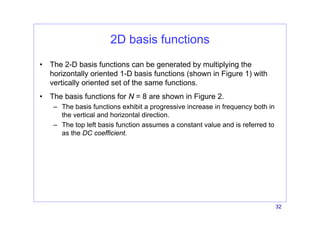
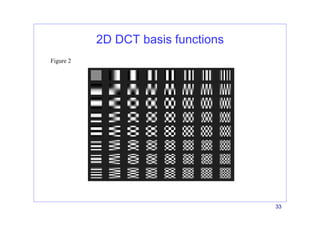
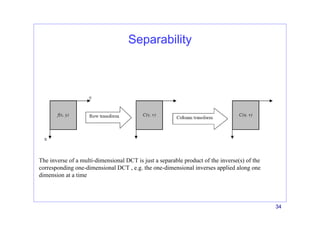
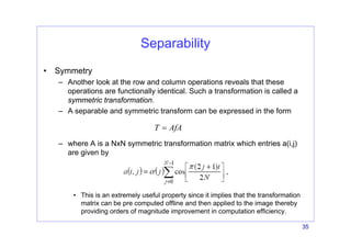
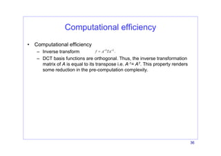
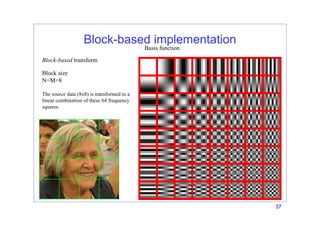
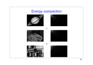
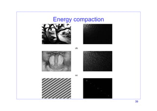
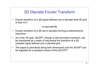
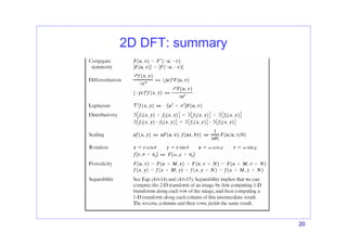
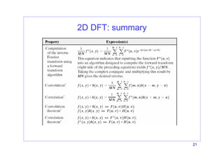
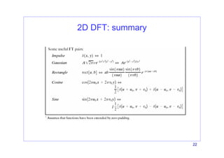
The document discusses the 2D discrete Fourier transform (DFT). It defines the 2D DFT and explains that it treats a 2D signal as periodic, resulting in periodicity properties. The 2D DFT can be computed as sequential 1D DFTs along rows and columns due to the separability of its basis functions. It also introduces the related 2D discrete cosine transform (DCT), which uses cosine basis functions.
![3
Circular convolution
• Finite length signals (N0 samples) → circular or periodic convolution
– the summation is over 1 period
– the result is a N0 period sequence
• The circular convolution is equivalent to the linear convolution of the
zero-padded equal length sequences
[ ]
f m
m
*
[ ]
g m
m
[ ]* [ ]
f m g m
m
=
Length=P Length=Q Length=P+Q-1
For the convolution property to hold, M must be greater than or equal to P+Q-1.
[ ]* [ ] [ ] [ ]
f m g m F k G k
⇔
0 1
0
[ ] [ ] [ ] [ ] [ ]
N
n
c k f k g k f n g k n
−
=
= ⊗ = −
∑](https://image.slidesharecdn.com/dftdcttransforms-231015114808-841d0b84/85/DFT-DCT-TRANSFORMS-pdf-3-320.jpg)
![4
Convolution
• Zero padding
[ ]* [ ] [ ] [ ]
f m g m F k G k
⇔
[ ]
f m
m
*
[ ]
g m
m
[ ]* [ ]
f m g m
m
=
[ ]
F k
4-point DFT
(M=4)
[ ]
G k [ ] [ ]
F k G k](https://image.slidesharecdn.com/dftdcttransforms-231015114808-841d0b84/85/DFT-DCT-TRANSFORMS-pdf-4-320.jpg)
![5
In words
• Given 2 sequences of length N and M, let y[k] be their linear convolution
• y[k] is also equal to the circular convolution of the two suitably zero padded
sequences making them consist of the same number of samples
• In this way, the linear convolution between two sequences having a different length
(filtering) can be computed by the DFT (which rests on the circular convolution)
– The procedure is the following
• Pad f[n] with Nh-1 zeros and h[n] with Nf-1 zeros
• Find Y[r] as the product of F[r] and H[r] (which are the DFTs of the corresponding zero-padded
signals)
• Find the inverse DFT of Y[r]
• Allows to perform linear filtering using DFT
[ ] [ ] [ ] [ ] [ ]
n
y k f k h k f n h k n
+∞
=−∞
= ∗ = −
∑
0 1
0
0
[ ] [ ] [ ] [ ] [ ]
+ 1: length of the zero-padded seq
N
n
f h
c k f k h k f n h k n
N N N
−
=
= ⊗ = −
= −
∑](https://image.slidesharecdn.com/dftdcttransforms-231015114808-841d0b84/85/DFT-DCT-TRANSFORMS-pdf-5-320.jpg)
![7
2D Discrete Fourier Transform (2D DFT)
• 2D Fourier (discrete time) Transform (DTFT) [Gonzalez]
2 ( )
( , ) [ , ] j um vn
m n
F u v f m n e π
∞ ∞
− +
=−∞ =−∞
= ∑ ∑
1 1 2
0 0
1
[ , ] [ , ]
k l
M N j m n
M N
m n
F k l f m n e
MN
π
⎛ ⎞
− − − +
⎜ ⎟
⎝ ⎠
= =
= ∑∑
• 2D Discrete Fourier Transform (DFT)
2D DFT can be regarded as a sampled version of 2D DTFT.
a-periodic signal
periodic transform
periodized signal
periodic and sampled
transform](https://image.slidesharecdn.com/dftdcttransforms-231015114808-841d0b84/85/DFT-DCT-TRANSFORMS-pdf-7-320.jpg)
![8
2D DFT: Periodicity
1 1 2
0 0
1
[ , ] [ , ]
k l
M N j m n
M N
m n
F k l f m n e
MN
π
⎛ ⎞
− − − +
⎜ ⎟
⎝ ⎠
= =
= ∑∑
1 1 2
0 0
1
[ , ] [ , ]
k M l N
M N j m n
M N
m n
F k M l N f m n e
MN
π
+ +
⎛ ⎞
− − − +
⎜ ⎟
⎝ ⎠
= =
+ + = ∑∑
1 1 2 2
0 0
1
[ , ]
k l M N
M N j m n j m n
M N M N
m n
f m n e e
MN
π π
⎛ ⎞ ⎛ ⎞
− − − + − +
⎜ ⎟ ⎜ ⎟
⎝ ⎠ ⎝ ⎠
= =
= ∑∑
1
• A [M,N] point DFT is periodic with period [M,N]
– Proof
[ , ]
F k l
=
(In what follows: spatial coordinates=k,l, frequency coordinates: u,v)](https://image.slidesharecdn.com/dftdcttransforms-231015114808-841d0b84/85/DFT-DCT-TRANSFORMS-pdf-8-320.jpg)
![9
2D DFT: Periodicity
• Periodicity
• This has important consequences on the implementation and energy
compaction property
– 1D
[ , ] [ , ] [ , ] [ , ]
F u v F u mM v F u v nN F u mM v nN
= + = + = + +
[ , ] [ , ] [ , ] [ , ]
f k l f k mM l f k l nN f k mM l nN
= + = + = + +
f[u]
u
M/2 M
0
[ ] [ ]
F N u F u
∗
− =
The two inverted periods meet here
f[k] real→F[u] is symmetric
M/2 samples are enough](https://image.slidesharecdn.com/dftdcttransforms-231015114808-841d0b84/85/DFT-DCT-TRANSFORMS-pdf-9-320.jpg)
![10
Periodicity: 1D
f[u]
u
M/2 M
0
It is more practical to have one complete period positioned in [0, M-1]
[ ] [ ]
f k F u
↔
0
0
2
0
2 2
2
0
[ ]e [ ]
e e e ( 1)
2
( 1) [ ] [ ]
2
u k
j
M
u k Mk
j j
j k k
M M
k
f k F u u
M
u
M
f k F u
π
π π
π
↔ −
= → = = = −
− ↔ −
changing the sign of every other
sample puts F[0] at the center of the
interval [0,M]
The two inverted periods meet here](https://image.slidesharecdn.com/dftdcttransforms-231015114808-841d0b84/85/DFT-DCT-TRANSFORMS-pdf-10-320.jpg)
![11
Periodicity: 2D
DFT periods
MxN values
4 inverted
periods meet
here
M/2
-M/2
N/2
-N/2
F[u,v]
(0,0)](https://image.slidesharecdn.com/dftdcttransforms-231015114808-841d0b84/85/DFT-DCT-TRANSFORMS-pdf-11-320.jpg)
![12
Periodicity: 2D
DFT periods
MxN values
4 inverted
periods meet
here
M/2
N/2
F[u,v]
(0,0) M-1
N-1
0 0
2 ( )
0 0
0 0
[ , ]e [ , ]
,
2 2
( 1) [ ] ,
2 2
u k v l
j
M N
k l
f k l F u u v v
M N
u v
M N
f k F u v
π +
+
↔ − −
= = →
⎡ ⎤
− ↔ − −
⎢ ⎥
⎣ ⎦
data contain one centered
complete period](https://image.slidesharecdn.com/dftdcttransforms-231015114808-841d0b84/85/DFT-DCT-TRANSFORMS-pdf-12-320.jpg)
![13
Periodicity: 2D
M/2
N/2
F[u,v]
(0,0) M-1
N-1
4 inverted
periods meet
here](https://image.slidesharecdn.com/dftdcttransforms-231015114808-841d0b84/85/DFT-DCT-TRANSFORMS-pdf-13-320.jpg)
![14
Periodicity in spatial domain
1 1 2
0 0
[ , ] [ , ]
k l
M N j m n
M N
k l
f m n F k l e
π
⎛ ⎞
− − +
⎜ ⎟
⎝ ⎠
= =
= ∑∑
1
• [M,N] point inverse DFT is periodic with period [M,N]
1 1 2 ( ) ( )
0 0
[ , ] [ , ]
k l
M N j m M n N
M N
k l
f m M n N F k l e
π
⎛ ⎞
− − + + +
⎜ ⎟
⎝ ⎠
= =
+ + = ∑∑
1 1 2 2
0 0
[ , ]
k l k l
M N j m n j M N
M N M N
k l
F k l e e
π π
⎛ ⎞ ⎛ ⎞
− − + +
⎜ ⎟ ⎜ ⎟
⎝ ⎠ ⎝ ⎠
= =
= ∑∑
[ , ]
f m n
=](https://image.slidesharecdn.com/dftdcttransforms-231015114808-841d0b84/85/DFT-DCT-TRANSFORMS-pdf-14-320.jpg)
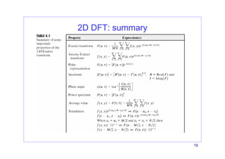
![15
Angle and phase spectra
[ ] [ ] [ ]
[ ] [ ]
{ } [ ]
{ }
[ ]
[ ]
{ }
[ ]
{ }
[ ]
,
1/ 2
2 2
2
, ,
, Re , Im ,
Im ,
, arctan
Re ,
[ , ] ,
j u v
F u v F u v e
F u v F u v F u v
F u v
u v
F u v
P u v F u v
Φ
=
⎡ ⎤
= +
⎣ ⎦
⎡ ⎤
Φ = ⎢ ⎥
⎣ ⎦
=
modulus (amplitude spectrum)
phase
power spectrum
For a real function
[ , ] [ , ]
[ , ] [ , ]
[ , ] [ , ]
F u v F u v
F u v F u v
u v u v
∗
− − =
− − =
Φ − − = −Φ
conjugate symmetric with respect to the origin](https://image.slidesharecdn.com/dftdcttransforms-231015114808-841d0b84/85/DFT-DCT-TRANSFORMS-pdf-15-320.jpg)
![16
Translation and rotation
[ ]
[ ] [ ]
2
2
[ , ] ,
, ,
m n
j k l
M N
m n
j k l
M N
f k l e F u m v l
f k m l n F u v
π
π
⎛ ⎞
+
⎜ ⎟
⎝ ⎠
⎛ ⎞
− +
⎜ ⎟
⎝ ⎠
↔ − −
− − ↔
[ ] [ ]
0 0
cos cos
sin sin
, ,
k r u
l r l
f r F
ϑ ω ϕ
ϑ ω ϕ
ϑ ϑ ω ϕ ϑ
= =
⎧ ⎧
⎨ ⎨
= =
⎩ ⎩
+ ↔ +
Rotations in spatial domain correspond equal rotations in Fourier domain](https://image.slidesharecdn.com/dftdcttransforms-231015114808-841d0b84/85/DFT-DCT-TRANSFORMS-pdf-16-320.jpg)
![17
mean value
[ ] [ ]
1 1
0 0
1
0,0 ,
N M
n m
F f n m
NM
− −
= =
= ∑∑ DC coefficient](https://image.slidesharecdn.com/dftdcttransforms-231015114808-841d0b84/85/DFT-DCT-TRANSFORMS-pdf-17-320.jpg)
![18
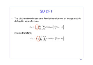
Separability
• The discrete two-dimensional Fourier transform of an image array is
defined in series form as
• inverse transform
• Because the transform kernels are separable and symmetric, the two
dimensional transforms can be computed as sequential row and column
one-dimensional transforms.
• The basis functions of the transform are complex exponentials that may be
decomposed into sine and cosine components.
1 1 2
0 0
1
[ , ] [ , ]
k l
M N j m n
M N
m n
F k l f m n e
MN
π
⎛ ⎞
− − − +
⎜ ⎟
⎝ ⎠
= =
= ∑∑
1 1 2
0 0
[ , ] [ , ]
k l
M N j m n
M N
k l
f m n F k l e
π
⎛ ⎞
− − +
⎜ ⎟
⎝ ⎠
= =
= ∑∑](https://image.slidesharecdn.com/dftdcttransforms-231015114808-841d0b84/85/DFT-DCT-TRANSFORMS-pdf-18-320.jpg)
![24
2D Discrete Fourier Transform
• Inverse DFT
1 1 2
0 0
1
[ , ] [ , ]
k l
M N j m n
M N
m n
F k l f m n e
MN
π
⎛ ⎞
− − − +
⎜ ⎟
⎝ ⎠
= =
= ∑∑
• 2D Discrete Fourier Transform (DFT)
1 1 2
0 0
[ , ] [ , ]
k l
M N j m n
M N
k l
f m n F k l e
π
⎛ ⎞
− − +
⎜ ⎟
⎝ ⎠
= =
= ∑∑
where
0,1,..., 1
k M
= −
0,1,..., 1
l N
= −](https://image.slidesharecdn.com/dftdcttransforms-231015114808-841d0b84/85/DFT-DCT-TRANSFORMS-pdf-24-320.jpg)
![25
2D Discrete Fourier Transform
• Inverse DFT
1 1 2
0 0
1
[ , ] [ , ]
k l
M N j m n
M N
m n
F k l f m n e
MN
π
⎛ ⎞
− − − +
⎜ ⎟
⎝ ⎠
= =
= ∑∑
• It is also possible to define DFT as follows
1 1 2
0 0
1
[ , ] [ , ]
k l
M N j m n
M N
k l
f m n F k l e
MN
π
⎛ ⎞
− − +
⎜ ⎟
⎝ ⎠
= =
= ∑∑
where 0,1,..., 1
k M
= −
0,1,..., 1
l N
= −](https://image.slidesharecdn.com/dftdcttransforms-231015114808-841d0b84/85/DFT-DCT-TRANSFORMS-pdf-25-320.jpg)
![26
2D Discrete Fourier Transform
• Inverse DFT
1 1 2
0 0
[ , ] [ , ]
k l
M N j m n
M N
m n
F k l f m n e
π
⎛ ⎞
− − − +
⎜ ⎟
⎝ ⎠
= =
= ∑∑
• Or, as follows
1 1 2
0 0
1
[ , ] [ , ]
k l
M N j m n
M N
k l
f m n F k l e
MN
π
⎛ ⎞
− − +
⎜ ⎟
⎝ ⎠
= =
= ∑∑
where and
0,1,..., 1
k M
= − 0,1,..., 1
l N
= −](https://image.slidesharecdn.com/dftdcttransforms-231015114808-841d0b84/85/DFT-DCT-TRANSFORMS-pdf-26-320.jpg)